A SEARCH ALGORITHM ON A RELATIONAL DATASET
CONTAINING ALGORITHMS TO FACILITATE REAL TIME
CODE GENERATION
1 SENTHIL JAYAVEL2S ARUMUGAM 3PRATIK SHAH 4RAHUL DE
1
Senior Asstt Prof., Department of Computer Science And Engineering, VIT University, Vellore, India
2
Assoc. Prof., Nandha University, Erode, Tamil Nadu, India
3 Student, School of Computer Science And Engineering, VIT University. Vellore, India 4 Student, School of Computer Science And Engineering, VIT University., Vellore, India
E-mail: [email protected]@yahoo.co.in3 [email protected]
ABSTRACT
The world of computation originates from 1’s, 0’s and the algorithms that work on sequences of these bits to generate outputs. Over the past half a century the world of computation has seen numerous algorithms and these algorithms have helped us solve our problems. These problems that we face are of a repetitive nature and we use these same algorithms to solve them repeatedly. We tend to always store the data that is essential to us and these algorithms are one of the most essentials things that help us get through day-to-day lives. This paper deals with the construction of a collection of algorithms in a structured relational database pattern to help us store the algorithms in an intuitive way and along with that this paper also deals with a search algorithm that works on this collection to give algorithms as output. These output algorithms can later be put to use in a number of domains as mentioned in the applications section of this paper.
Keywords: Relational Database, Algorithm, Search, Relevance Factor, Graphs, Weights, Nodes, Edges.
1.
INTRODUCTIONBefore we go to the search algorithm we shall talk about the construction of the collection of the algorithms into a relational database. For all purposes this collection will be further called as a dataset. The dataset is a connected graph in which the nodes consist the algorithms and other parameters and the connected nodes have an edge with one or multiple weights. Once the dataset has been constructed new nodes can be added and modified and replaced easily.
The major feature of this dataset is that it can continuously grow and it can be continuously updated as at the very base of this dataset is nothing but a graph which can be vey easily changed, modified and updated and by making the dataset open, the very same operations can be performed on the dataset by anyone in this world. This makes it readily available to every one for use as well as provides a ready base for making one’s algorithm available to everyone for use.
The search algorithm works on this dataset and based on the input keywords it searches for one or more algorithms that have the greatest relevance hit in the solving the problem that is defined by the
input keywords. These algorithms are given as the output of the search, which can be put to further use. The search algorithm also takes constraints of the algorithms into considerations and the total relevance hit is calculated and based on it the algorithm is searched and given as the input.
2.
DATASETThe dataset i.e. the collection of all the algorithms in a relational model must be constructed, as the dataset on its own is one of the inputs to the search algorithm that will give a relevant algorithm as the output. The construction of the dataset uses the concepts of graphs and thus invariably uses nodes and edges. The nodes are used to store all the information and the edges which shall be weighted and
undirected will be used to store the relationship between two nodes or rather two algorithms.
The relational dataset is an undirected tree, which can be defined mathematically as follows
Where n is the total number of vertices present inside the dataset.
E = {ei; 1 ≤ i ≤ n-1: ∀ei, ei.v1∈V & ei.v2∈V}
Where v1 is start node for that edge and v2 is the
node on which that edge is incident.
W = {wi; 1 ≤i ≤ n-1: ∀wi, wi← ei.w}
Where each wi is a set of keywords.
2.1. Structure Of The Nodes Vi
Before going into the structure of the dataset we must first define the structure of the nodes that the dataset will contain. The nodes will consist of two entities, the algorithm file and the names of the authors. The algorithms must all be present in a readable text file and they must all be written in the structure provided below.
• Each algorithm must begin with ‘Start’ as the first step and ‘Stop’ as the last step.
• Each step must be given sequential numbers without any special characters. E.g. ‘1’, ‘2’, ‘3’ etc.
• Each sub-step must be given roman numbering in lower case without any special characters e.g. ‘i’, ‘ii’ etc.
General rules that must be followed in the algorithm file are
• The algorithm should be written in clear, crisp steps.
• There should be no ambiguity in the algorithm.
• All the definitions and the declarations must be properly given.
The combination of the author names and the file that contains the algorithm forms the contents of a particular node in the graph.
2.2 Structure Of The Edges
The nodes are connected using edges. These edges are weighted but not with numerical weights. The weights on a particular edge will be the keywords that form the relation from one node to the other. With the formal definition given above for the edge set of G
E = {ei; 1 ≤ i ≤ n-1: ∀ei, ei.v1∈V & ei.v2∈V}
Where v1 is start node for that edge and v2 is the
node on which that edge is incident.
We can clearly see that every edge ei will consist
of three parameters, which are v1, v2 and the
pointer to the set of weights wi.
The keywords that are present in wi are the
keywords that join v1 to v2. This relation states
that the algorithm solved by v2 solves some more
additional problems described by the keywords in wi than v1.
Each edge represents a unique relation and all edges are unique. The intersection of weights of different edges may or may not be disjoint and each and every node represents a single algorithm. Before we move on to the algorithm for the creation of the dataset or the search algorithm on the dataset we will first have a look at three functions which play a significant role in both the algorithm for creation of the dataset as well as the algorithm to search for an algorithm stored inside the dataset.
2.3 Working Of The Dataset
For the dataset to be created as well as to be searched we need keywords. These keywords are nothing but a specific set of words that define the problem that is to be added to the dataset or it defines the problem for which an algorithm is being searched from the dataset. This set of keywords can be denoted mathematically as
K = {ki; 1 ≤ i ≤ m}
Using these keywords the entire dataset will be searched to find the place to add the new algorithm or to find the node/nodes that contain the algorithm/s that will be used to solve the problem defined by the keywords.
The three major functions that are called in sequence to find that place or the nodes are as follows.
2.3.1 Function to extract the subgraphs from the dataset
This function does the following jobs
• It finds all the edges from the tree G such that at least one of the weights on each edge matched with at least one keyword.
• From the set of edges that have been computed from step one it stiches these edges into one or multiple subgraphs.
This function uses many sets that have been defined below,
K = {ki; 1 ≤ i ≤ m} – This is the set of the input
S = {ei; 1 ≤ i < n-1 | (∃ki ∈ K) ∈ ei.w} – This set
is the set of all the edges in G such that at least one of the weights on each of those edges has at least matching keyword in K.
G’ = {Gi’; ∀Gi’ = {V’, E’} | Gi’ ⊆ G} – This is a
set of all the subgraphs that are formed form the edges that are present in S
A = {vi | ∀vi, vi = ei.v2 where ei ∈ S} – This is the
set of all the vertices that have the edges of S as their incident edges. These vertices contain the algorithm that is able to define the problem defined by K at least partially as each and every one of those vertices has at least one of the keywords matching with K.
B’ = {Bi}; Bi = {{longest}, {klist}},where longest
= the longest relevance path in the Gi’ subgraph &
klist = the list of all the keywords on the path on longest
The algorithm to find the subgraphs can be defined as follows
extractSubgraphs() {
S’ = {};
∀Gi’, Gi’.V’ = {}, Gi’.E’ = {}; V’’ = {};
ex = e1 //e1 is
the first edge in the set S
j = 1; do {
vx = ex.v1;
Gj’.V’ = Gj’.V’ ∪ {vx}; for ∀vi ∈ Gj’.V’ && ∀vi ∉ V’’ {
S’ = {el; 1 ≤ l < n-1 |
el.v1 = vx, ∀ei ∈ S}; Gj’.E’ = Gj’.E’ ∪ S’;
Gj’.V’ =
Gj’.V’ ∪ {vl : vl = el.v2};
S = S – S’; S’ = {}; }
V’’ = Gj’.V’ ∪ V’’;
ex = {e| e.v2 = vx}; if(ex= Φ & |S| ≠ 0) {
headj = vx j++; ex = e1; }
}while(|S| ≠ 0); }
2.3.1.1 Tme complextity
The above algorithm forms a crucial part of all the algorithms for the dataset and thus its time complexity lends a significant part to the time complexity of those other algorithms and thus the time complexity of the above algorithm must be calculated.
To calculate the worst case time complexity we will assume that at every for all factors that can contribute to the runtime of the above algorithm the size of that factor is N which is very large.
• We know that every ∀ will take O(N)
time complexity
• We know that every ∪ will take O(N2)
time complexity as in every addition to the set we must first ensure that it does not already exist in the set to which it being added.
Using the above two rules and the standard rules of finding the time complexity in the worst case we can calculate the total worst-case time complexity.
The above algorithm has the time complexity as calculated below
• do - while loop – O(N) • for - loop – O(N)
• A block of statements – O(1)
O(1) + (O(N) * (O(1) + O(N) + (O(N) * (O(1) +
O(N2) + O(N2))) + O(N2) + O(1))) (1)
= O(1) + (O(N) * (O(N) + (O(N) * O(N2)) +
O(N2)))
= O(1) + ((O(N) * O(N3)) + O(N2) = O(1) + O(N4) + O(N2)
Thus we can conclude that even in the worst case scenario the algorithm runs in polynomial time complexity.
2.3.1.2 Explanation
In the above algorithm the edges that have weights that match the keywords that have been given by the user are computed and then these edges are used to create the subgraphs.
• The first computed edge is taken
• The first node of this edge is taken as the initial node in the subgraph
• All the computed nodes are searched for the edges that have the same first node as the initial node.
• All these edges along with their second nodes are added to the subgraph
• This process is repeated for all the nodes that are in the subgraph.
• Once out of the for loop we calculate if the subgraph is yet to be complete by checking if the initial node is the second node for any of the edge in the set of computed edges. If yes then the first node of that node becomes the initial node and the process is repeated. Else if there are still some edges left in the computed set of edges then we make the next subgraph.
We repeat all the above steps till the computed edge is not empty.
2.3.2 Function to find the longest chain in the graph
The second algorithm that is used in all the algorithms for the data set is given below.
longestChain() {
for ∀Gi’ ∈ G’ {
DFS(Gi’.head, i); }
}
DFS(start, i) {
list = {};
count = 0, last = 0; for ∀child ∈ start.children {
list.append(child); if(child.children = Φ) {
if(count>last) {
Bi.longest=list; last = count; count = 0; }
else {
count+=max(K,child,i) DFS(child.children); }
} }
max(K, child, i) {
c = 0; for ∀ki∈ K {
for ∀k ∈ child.keywords {
if(k == ki) {
if(!Bi.klist.contain(k|”same”)){
Bi.klist.append(k); c++;}
} }
} return c; }
2.3.2.1 Time complexity
To calculate the time complexity we need to calculate the time complexity of the DFS() and to calculate the time complexity of DFS() we need to calculate the time complexity of the max function.
The time complexity of the max() function
O(1) + (O(N)*O(1)) (2)
= O(1) + O(N) = O(N)
(Result 2)
The time complexity of the DFS() function
O(N) * (O(1) + (O(N)*(O(1) + (max(O(1), (O(N))) (3)
= O(N) * (O(1) + O(N2)) = O(N) * O(N2) = O(N3)
As the recursive call happens N times the entire time complexity is multiplied by O(N) and thus we get O(N3)
The time complexity of the longestChain() function is
O(N)*O(N3) = O(N4)
Thus we can conclude that longestChain() has a polynomial time worst case time complexity.
2.3.2.2 Explanation
In the function for longestChain() a depth first search is run on each of the subgraphs that we computed to calculate the longest weighted path in them. Here the weights would be the total number weights in the path that match with the keywords. This function results in two sets; one, which contains the vertices of the path and the other contains all the keywords encountered in that path.
2.3.3 Function to sort the paths that have been found
The third function is described below
sortPaths() {
for ∀Bi∈ B’ {
for ∀Bj∈ B’ – {Bi} {
if(|Bi.klist|<|Bj.klist|) Bi↔ Bj }
} }
2.3.3.1 Time complexity
O(N)*(O(N)*(O(1)) (4)
= O(N)*O(N) = O(N2)
(Result 4)
Thus the function sortPaths() has a polynomial time worst case run time complexity.
2.3.3.2 Explanation
This function is used to sort the longest paths of all the subgraphs in descending order.
2.4 Creation Of The Dataset
The dataset creation is one of the most important processes related to the dataset as it includes adding new algorithms, or replacing previous algorithms etc. Since both these processes are processes that will still take place even after the dataset is created hence this algorithm plays a major role. Apart from that this algorithm helps in building the entire tree that is the dataset.
In this algorithm an input node is provided along with a set of keywords that best define the problem that is solved by the algorithm given in the input node.
2.4.1 The algorithm create()
{
extractSubgraphs(); longestChain(); sortPaths(); K = K – B1.klist;
Vs = B1.longest[|longest|-1]; Vi = getInput();
if(K = Φ) {
if(Vi.author = Vs.author) Vi↔ Vs
else {
V = V ∪ {Vi};
E = E ∪ {e| e.V1 = Vs & e.V2 = Vi & e.w = “same”};
} }
else {
V = V ∪ {Vi};
E = E ∪ {e| e.V1 = Vs & e.V2 = Vi & e.w = K};
W = W ∪ {wi = K}; }
}
2.4.1.1 Time complexity
O(N4) + O(N4) + O(N2) + max(O(1), O(N) +
O(N), O(N) + O(N) + O(N)) (5)
= O(N4) + O(N) = O(N4).
(Result 5)
Thus we can conclude that create() function has a polynomial time run time complexity in its worst case scenario. Thus each and every operation of addition of a node or modification of a node in the dataset takes polynomial time to execute and since the creation of the dataset is a collection of these polynomial operations the creation of the entire dataset also takes polynomial time complexity hence the creation of the dataset belongs the P problem.
2.4.1.2 Explanation
In this algorithm the previously defined functions are used to find the place where the input node will be attached. Once we get the longest chains of all the subgraphs we sort it in a way such that the first longest chain is the chain that has matched the maximum number of keywords with the keywords given in the input and thus the new node has to be attached to this very chain. If all the keywords have been matched then it must mean that the input node contains another version of the algorithm that already exists in the dataset. If the author of the last node in the chain and the author of the new node is the same then it means that the author has uploaded a new version of his/her algorithm and thus it is replaced else if it is from a different author then it is considered as a different version of the algorithm and added to the last node of the longest chain with the edge having the keyword as same which states that the algorithm is similar to its parent. If all the keyword have not been matched then we add the node to the end of the chain.
2.5 Searching In The Dataset
The main purpose of creating such a dataset is so that it can provide various applications by providing us with algorithms that can help us solve many problems. However for that to work we need a searching algorithm on this dataset that given a set of keywords that define the problem that the user is having the using those set of keywords the search algorithm must be able to give a number of plausible solutions in the form of algorithms and all these solutions must be ranked to make it user friendly.
The proposition of one such algorithm is given below. It takes a set of input keywords and thereby with the help of that it searches for the algorithms.
2.5.1 Ehe algorithm search(K)
{
extractSubgraphs(); longestChain(); sortPaths(); for ∀Bi∈ B’ {
output(Rank i, Bi.longest); }
output(lowest_rank, A); }
2.5.2 Time complexity
Using the results for of time complexity calculated for the previous functions we can calculate the time complexity of this function.
O(N4) + O(N4) + O(N2) + O(N) + O(1) (6) = O(N4)
(Result 6)
Thus we can conclude that the search function takes polynomial time complexity in the worst-case scenario. Thus the problem of finding an algorithm from the dataset belongs to the P class of the problem.
2.5.1.2 Explanation
To search the algorithm we need to find the nodes that match the constraints that are set by the keywords. The functions defined previously help us in achieving the exact same thing. As we get the longest chains consisting of nodes that satisfy the maximum number matches with the given keywords and also the function sortPaths() sorts all the paths such that the first path is the one that has the maximum matches with the given inputs. The final set A is also given as output as the set A consists of all the nodes that match at least one of the constraints set forth by the keywords.
In this manner the dataset is created and the search can be also used to get the algorithms as the output.
This kind of dataset provides a lot of applications however in this paper we shall deal only with two of the major applications.
3.1. A Search Engine for Algorithms
This application is one of the most evident applications of this kind of the dataset. This dataset provides one of the first and unique search engines specifically for algorithms as you can add as well as search for algorithms using this kinds of dataset.
3.2. Real Time Generative Programming
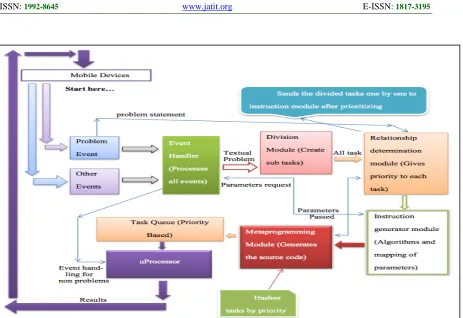
The major feature of this kind of application is that it provides algorithms as output. In a real time generative programming model provided in a paper “Real Time Code Generation using Generative Programming Paradigm” in the European Journal of Scientific Research the author provides a model for metaprogramming that is used to code the problem after an algorithm for that problem has been received, Using this algorithm the metaprogramming module codes step by step the entire code to the problem. The constraints given in this paper for writing the algorithm are for this singular purpose as that way of writing the algorithm helps the metaprogramming module to code the program for the problem given by the user.
FIGURE 1. [GIVEN IN THE ANNEXURE]
4.
CONCLUSIONThe creation of a relational dataset that can hold the algorithm is one of the first works that provides the basis to move in a direction in which we can reach a place where machines can solve problems by interacting with them as we interact with each other on a daily basis. By using many paradigms such as Natural Language Processing, Generative Programming and the dataset we can build machines that are able to interact with us in the most human way possible. Other than that, this dataset and the algorithms provides one of the first search engines for algorithms and thus a common platform to spread algorithms as well as a common platform to search for algorithms that can help developers and coders everywhere to develop better code.
REFRENCES:
[1] Levandoski, J.J., RDF Data-Centric Storage in
Web Services, 2009. ICWS 2009. IEEE International Conference on -10 July 2009 6 . Appears in pages 911 – 918.
[2] Senthil, J., Arumugam, S., Shah, Pratik., Real Time Code Generation Using Generative Programming Paradigm in European Journal of Scientific Research Volume 78, Issue 4, June 2012, Pages 581-587.
[3] Bollegala, D., A supervised ranking approach for detecting relationally similar word pairs in
Information and Automation for Sustainability (ICIAFs), 2010 5th International Conference
on 17-19 Dec. 2010, appears in pages 323 –
328.
[4] Liang Zhu, Yong Zhu, Qin Ma, Chinese Keyword Search over Relational Databases in
Software Engineering (WCSE), 2010 Second
World Congress on, 19-20 Dec. 2010, appears
in pages 217 - 220
[5] Liang Zhu, Shen-Da Ji, Wen-Zhu Yang, Chun-Nian Liu, Keyword search based on knowledge base in relational databases in
Machine Learning and Cybernetics, 2009 International Conference on 12-15 July 2009
5. ANNEXURE
Figure 1. A Model Of Real Time Generative Programming Given In European Journal Of Scientific Research