SRC RR 82 pdf

82

A Guide to LP, The Larch

Prover

Stephen J. Garland and John V. Guttag

Systems Research Center

DEC’s business and technology objectives require a strong research program. The Systems Research Center (SRC) and three other research laboratories are committed to filling that need.

SRC began recruiting its first research scientists in l984—their charter, to advance the state of knowledge in all aspects of computer systems research. Our current work includes exploring high-performance personal computing, distributed computing, programming environments, system modelling techniques, specification technology, and tightly-coupled multiprocessors.

Our approach to both hardware and software research is to create and use real systems so that we can investigate their properties fully. Complex systems cannot be evaluated solely in the abstract. Based on this belief, our strategy is to demonstrate the technical and practical feasibility of our ideas by building prototypes and using them as daily tools. The experience we gain is useful in the short term in enabling us to refine our designs, and invaluable in the long term in helping us to advance the state of knowledge about those systems. Most of the major advances in information systems have come through this strategy, including time-sharing, the ArpaNet, and distributed personal computing.

SRC also performs work of a more mathematical flavor which complements our systems research. Some of this work is in established fields of theoretical computer science, such as the analysis of algorithms, computational geometry, and logics of programming. The rest of this work explores new ground motivated by problems that arise in our systems research.

DEC has a strong commitment to communicating the results and experience gained through pursuing these activities. The Company values the improved understanding that comes with exposing and testing our ideas within the research community. SRC will therefore report results in conferences, in professional journals, and in our research report series. We will seek users for our prototype systems among those with whom we have common research interests, and we will encourage collaboration with university researchers.

A Guide to LP, The Larch Prover

Stephen J. Garland and John V. Guttag

John V. Guttag and Stephen J. Garland are at the MIT Laboratory for Computer Science, 545 Technology Square, Cambridge, MA 02139.

E-mail: [email protected], [email protected]

The authors were supported in part by the Advanced Research Projects Agency of the Department of Defense, monitored by the Office of Naval Research under contract N00014-89-J-1988, by the National Science Foundation under grant CCR-8910848, and by the Digital Equipment Corporation.

c

Abstract

Contents

1 Introduction 1

2 The proof life cycle 2

3 Getting started 4

3.1 Typesetting conventions : : : : : : : : : : : : : : : : : : : : : : : : : : : : : : : : : 4 3.2 Online help: : : : : : : : : : : : : : : : : : : : : : : : : : : : : : : : : : : : : : : : 4

3.3 Entering commands : : : : : : : : : : : : : : : : : : : : : : : : : : : : : : : : : : : 5 3.4 Naming and displaying objects: : : : : : : : : : : : : : : : : : : : : : : : : : : : : : 6

3.5 Recording sessions: : : : : : : : : : : : : : : : : : : : : : : : : : : : : : : : : : : : 7

3.6 Settings : : : : : : : : : : : : : : : : : : : : : : : : : : : : : : : : : : : : : : : : : 7

4 Defining theories 9

4.1 Declarations and identifiers : : : : : : : : : : : : : : : : : : : : : : : : : : : : : : : 9 4.2 Terms : : : : : : : : : : : : : : : : : : : : : : : : : : : : : : : : : : : : : : : : : : 10

4.3 Equations : : : : : : : : : : : : : : : : : : : : : : : : : : : : : : : : : : : : : : : : 11

4.4 Rewrite rules : : : : : : : : : : : : : : : : : : : : : : : : : : : : : : : : : : : : : : : 12 4.5 Operator theories: : : : : : : : : : : : : : : : : : : : : : : : : : : : : : : : : : : : : 14

4.6 Induction rules : : : : : : : : : : : : : : : : : : : : : : : : : : : : : : : : : : : : : : 15 4.7 Deduction rules : : : : : : : : : : : : : : : : : : : : : : : : : : : : : : : : : : : : : 16

4.8 Built-in operators and axioms : : : : : : : : : : : : : : : : : : : : : : : : : : : : : : 17

4.9 Orienting equations into rewrite rules : : : : : : : : : : : : : : : : : : : : : : : : : : 18

4.9.1 Registered orderings: : : : : : : : : : : : : : : : : : : : : : : : : : : : : : : 19 4.9.2 Polynomial orderings : : : : : : : : : : : : : : : : : : : : : : : : : : : : : : 20

4.9.3 Brute-force orderings : : : : : : : : : : : : : : : : : : : : : : : : : : : : : : 21 4.9.4 Interacting with the ordering procedures: : : : : : : : : : : : : : : : : : : : : 21

5 Forward inference in LP 23

5.1 Normalization : : : : : : : : : : : : : : : : : : : : : : : : : : : : : : : : : : : : : : 23

5.2 Application of deduction rules : : : : : : : : : : : : : : : : : : : : : : : : : : : : : : 23

5.3 Critical-pair equations : : : : : : : : : : : : : : : : : : : : : : : : : : : : : : : : : : 23 5.4 Completion: : : : : : : : : : : : : : : : : : : : : : : : : : : : : : : : : : : : : : : : 25

5.5 Instantiation : : : : : : : : : : : : : : : : : : : : : : : : : : : : : : : : : : : : : : : 26

6 Backward inference in LP 29

6.1 Proofs by normalization : : : : : : : : : : : : : : : : : : : : : : : : : : : : : : : : : 30

6.2 Proofs by cases: : : : : : : : : : : : : : : : : : : : : : : : : : : : : : : : : : : : : : 31 6.3 Proofs by induction : : : : : : : : : : : : : : : : : : : : : : : : : : : : : : : : : : : 32

6.4 Proofs by contradiction : : : : : : : : : : : : : : : : : : : : : : : : : : : : : : : : : 34

6.5 Proofs of implications : : : : : : : : : : : : : : : : : : : : : : : : : : : : : : : : : : 34

6.6 Proofs of conditionals : : : : : : : : : : : : : : : : : : : : : : : : : : : : : : : : : : 35 6.7 Proofs of conjunctions : : : : : : : : : : : : : : : : : : : : : : : : : : : : : : : : : : 35

6.8 Proofs by explicit commands: : : : : : : : : : : : : : : : : : : : : : : : : : : : : : : 35 6.9 Default proof methods : : : : : : : : : : : : : : : : : : : : : : : : : : : : : : : : : : 35

6.10 Proofs of deduction rules: : : : : : : : : : : : : : : : : : : : : : : : : : : : : : : : : 36

6.11 Proofs of induction rules : : : : : : : : : : : : : : : : : : : : : : : : : : : : : : : : : 36

7 Features of LP 37

7.1 Commands for user interaction: : : : : : : : : : : : : : : : : : : : : : : : : : : : : : 37 7.1.1 Saving and restoring state : : : : : : : : : : : : : : : : : : : : : : : : : : : : 38

7.1.2 Displaying information : : : : : : : : : : : : : : : : : : : : : : : : : : : : : 38

7.3 Commands for proving theorems: : : : : : : : : : : : : : : : : : : : : : : : : : : : : 42 7.3.1 Proof methods : : : : : : : : : : : : : : : : : : : : : : : : : : : : : : : : : : 43

7.3.2 Box checking : : : : : : : : : : : : : : : : : : : : : : : : : : : : : : : : : : 43 7.4 Commands for ordering equations into rewrite rules : : : : : : : : : : : : : : : : : : : 43

7.5 Settings : : : : : : : : : : : : : : : : : : : : : : : : : : : : : : : : : : : : : : : : : 44

7.5.1 Settings that affect output : : : : : : : : : : : : : : : : : : : : : : : : : : : : 46

7.5.2 Settings that affect rewriting : : : : : : : : : : : : : : : : : : : : : : : : : : : 46

8 Hints on using LP 47

8.1 Preparing input and recording work : : : : : : : : : : : : : : : : : : : : : : : : : : : 47 8.2 Formalizing axioms and conjectures : : : : : : : : : : : : : : : : : : : : : : : : : : : 47

8.3 Ordering equations into rewrite rules: : : : : : : : : : : : : : : : : : : : : : : : : : : 48 8.4 Managing proofs : : : : : : : : : : : : : : : : : : : : : : : : : : : : : : : : : : : : : 49

8.5 Making proofs go faster : : : : : : : : : : : : : : : : : : : : : : : : : : : : : : : : : 50

8.6 Overcoming installation problems : : : : : : : : : : : : : : : : : : : : : : : : : : : : 50 8.7 Reporting bugs: : : : : : : : : : : : : : : : : : : : : : : : : : : : : : : : : : : : : : 50

9 Current development 52

10 Acknowledgements 53

Appendices

54

A Equational term-rewriting tutorial 54

A.1 Equational theories: : : : : : : : : : : : : : : : : : : : : : : : : : : : : : : : : : : : 54

A.2 Term-rewriting systems : : : : : : : : : : : : : : : : : : : : : : : : : : : : : : : : : 55 A.3 Unification : : : : : : : : : : : : : : : : : : : : : : : : : : : : : : : : : : : : : : : : 55

A.4 Critical pairs : : : : : : : : : : : : : : : : : : : : : : : : : : : : : : : : : : : : : : : 56

A.5 Completion: : : : : : : : : : : : : : : : : : : : : : : : : : : : : : : : : : : : : : : : 57 A.6 Proving termination : : : : : : : : : : : : : : : : : : : : : : : : : : : : : : : : : : : 58

A.6.1 Simplification orderings : : : : : : : : : : : : : : : : : : : : : : : : : : : : : 59 A.6.2 Registered orderings: : : : : : : : : : : : : : : : : : : : : : : : : : : : : : : 59

B Sample proof 61

1

Introduction

LP is a theorem prover for a subset of multisorted first-order logic. It is designed to work efficiently on large problems and to be used by relatively naive users. It has been used to analyze formal specifications written in Larch [14, 15, 12], to reason about algorithms involving concurrency [10, 30], and to establish the correctness of hardware designs [10, 28].

LP is intended primarily as an interactive proof assistant or proof debugger, not as a fully automatic theorem prover. Its design is based on the assumption that initial attempts to state conjectures correctly, and then to prove them, usually fail. As a result, LP is designed to carry out routine (and possibly lengthy) steps in a proof automatically and to provide useful information about why proofs fail, if and when they do. To ensure that users will not be surprised by its behavior, LP does not employ complicated heuristics for finding proofs automatically. It does make it easy for users to employ standard techniques such as proofs by cases, induction, or contradiction.

Section 2 provides a context for the technical details of LP (Release 2.2) by discussing the style of use that LP is intended to support. Section 3 tells how to get started using LP. Section 4 describes how theories are axiomatized in LP. Sections 5 and 6 describe LP’s proof techniques. Section 7 summarizes the features of LP, and Section 8 provides some hints for using LP. Appendix A contains a tutorial on the theory and implementation of equational term-rewriting. Appendix B contains a complete record of a sample proof carried out using LP.

2

The proof life cycle

Proving is similar to programming: proofs are designed, coded, and debugged. The first step in designing a proof is to formalize the objects being reasoned about. The next is to formalize a conjecture to be proved, for example, a property implied by a specification, or an invariant to be maintained by a concurrent algorithm. The last step in the design is to outline a structure for the proof, including key lemmas and methods of proof.

Formalization is straightforward for Larch Shared Language [15] specifications and has been automated [12]. At present it is less automatic for concurrent algorithms and for circuits, although efforts are underway to automate some of these translations [30, 21]. For large applications, formalization usually involves identifying subtheories that are analogous to data abstractions. Generally, the most difficult design step, and the one requiring the most insight, is determining the structure of the proof.

Designs for proofs translate into sequences of LP commands, much as program designs translate into code in a programming language. Details of this translation are discussed later in this guide.

Once part of a proof has been coded, LP can be used to debug it. Proofs of interesting conjectures hardly ever succeed the first time. Sometimes the conjecture is wrong. Sometimes the formalization is incorrect or incomplete. Sometimes the proof strategy is flawed or not detailed enough. When an attempted proof does fail, a variety of LP facilities (e.g., case analysis) can be used to understand the problem. Because most proof attempts do fail, LP is designed to fail relatively quickly and to provide useful information when it does.

LP is not designed to find difficult proofs automatically. Unlike the Boyer-Moore prover [3, 4], it does not use heuristics to formulate additional conjectures that might be useful in a proof. Unlike LCF [24] and Isabelle [25], it does not encourage users to define their own proof tactics; rather, it provides a set of standard tactics and simple mechanisms for controlling the application of these tactics. Strategic decisions, such as trying induction on a particular variable, must appear as explicit LP commands (either entered by the user or generated by an application-specific front-end to LP). But LP is more than a proof checker, since it does not require proofs to be described in minute detail. Hence it is best described as a proof debugger.

In line with LP’s emphasis on debugging proofs, it is generally advisable to use axiomatizations that simplify terms rather than axiomatizations that produce unique (but possibly larger) normal forms. Such axiomatizations are often incomplete, and thereby increase the need for the kinds of auxiliary proof mechanisms described in Sections 5 and 6.

set name nat declare sort Nat

declare variables i;j;k: Nat

declare operators 0:!Nat s: Nat!Nat

C: Nat, Nat!Nat

<: Nat, Nat!Bool

..

assert Nat generated by 0, s assert acC

assert

iC0DDi

iCs.j/DDs.iCj/ not.i<0/

0<s.i/

s.i/ <s.j/DDi <j

..

set name lemma

prove i < j )i< .jCk/by induction on j <>2 subgoals for proof by induction on ‘ j ’

[ ] basis subgoal

resume by induction on i

<>2 subgoals for proof by induction on ‘i’ [ ] basis subgoal

[ ] induction subgoal [ ] induction subgoal [ ] conjecture

qed

Figure 1: Sample LP-annotated script file

might, for example, apply a tactic that the user intended for the basis step of an induction to the proof of the induction step. This checking helps prevent proofs from getting “out of sync” with their author’s conception of how they should proceed.

3

Getting started

This section describes how to use elementary LP features for entering commands and displaying information.

3.1

Typesetting conventions

This guide has been typeset using LaTeX [20]. Most of the examples of LP input and output in this guide have been preprocessed so that they are typeset using the following conventions.

ž LP command names and other keywords are printed in boldface (e.g., assert, display, generated by, induction, set).

ž Identifiers (see Section 4.1) are printed in italics (e.g., Bool, false, x, x1), except for numerals (e.g., 0, 1).

ž Names of facts and conjectures (see Section 3.4) are printed in italics (e.g., nat.1, lemmaCaseHyp.2). ž Names of files (see Sections 3.3 and 3.5) are printed in italics.

ž The following multicharacter symbols are printed using special non-ASCII characters.

Symbol Printed as

-> !

=> )

<=> ,

\in 2

\union [

\subseteq

<=

>= ½

If you prepare input for LP based on the examples in this guide, you must enter the special symbols in the right column of the table using the ASCII forms in the left column. While->,=>, and<=>are built-in symbols of LP (see Sections 4.1 and 4.8), the infix operator symbols\in,\union,\subseteq, and <=must be declared before use (see Section 4.1). The symbol>=has a built-in meaning to the register height command (see Section 4.9.1), but is not predeclared as an infix operator. Both it and the symbol <=must be declared before use (see Section 4.1) and have no built-in semantics.

3.2

Online help

Much of the information in this guide is also available from LP’s online help facility.1 The command help lp provides an overview of this facility. In general, users can type help followed by a list of topics for which they desire help. The command help ? provides a list of all topics for which help is available.

In most cases when LP expects input, users can type a question mark to obtain a summary of the legal responses. For example, the command ? produces a list of all LP commands, and the command assert ? provides a summary of the kinds of axioms that can be asserted.

3.3

Entering commands

LP generally prompts users to enter commands interactively from the keyboard. Users can also create files containing sequences of commands and instruct LP to execute these command files; for example, the command execute nat causes LP to execute the commands in the file nat.lp. (By convention, LP command files have names ending with .lp, and LP supplies .lp as a default suffix when no suffix appears in the execute command.) Command files may themselves contain execute commands; however, to guard against infinite loops, LP treats execution of a file that is already being executed as an error. Execution of a command file continues until the file is exhausted, until execution is interrupted by the user, until an error occurs, or until a quit or stop command is executed.

When run under Unix, LP can also be invoked with the names of one or more command files given as optional arguments. For example, the Unix shell command lp nat causes LP to start by executing the commands in the file nat.lp, and then to prompt the user for input when that file is exhausted.

All LP commands begin with a keyword (e.g., display or critical-pairs), which can be abbreviated to any unambiguous prefix (e.g., dis or crit). Some LP commands contain further keywords or phrases, which can also be abbreviated. For example, set automatic-ordering off can be shortened to set auto-ord off. Commands can be entered in upper, lower, or mixed case.

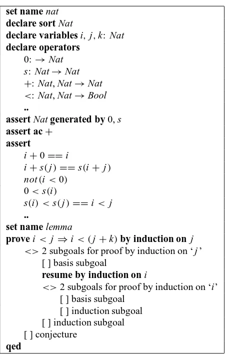
When an LP command requires more arguments than a user supplies, LP will prompt the user for the missing arguments. Users who need help can type a question mark followed by a carriage return to see what LP expects next; typing a carriage return alone aborts the command. If a missing argument is likely to be lengthy, LP prompts the user to enter it on subsequent lines and to terminate the input with a line consisting of two periods (..), which can be preceded by white space. The declare and assert commands in Figure 1 use this convention.

A comment starting with a % can occur at the end of any line of input or on a line by itself. LP ignores comments.

The following editing capabilities are available for use when typing input to LP. Editing character Action

rubout Delete last character typed control-U Delete current line of input control-R Redisplay current line

control-L Clear screen and redisplay current line control-n Continue line

Typing a control-G causes LP to interrupt execution of the current command.2 _{The quit command causes}

LP to terminate.

Induction rules:

nat.1: Nat generated by 0, s

Operator theories: nat.2: ac +

Rewrite rules:

lemma.1: (i < j) => (i < (j + k)) -> true nat.3: 0 + i -> i

nat.4: s(j) + i -> s(i + j) nat.5.1: i < 0 -> false nat.6: 0 < s(i) -> true nat.7: s(i) < s(j) -> i < j

Figure 2: Output generated by display command

3.4

Naming and displaying objects

The set name command provides users with control over the names assigned to facts (i.e., to axioms, hypotheses, and theorems) and to conjectures. For example, the command set name nat in Figure 1 causes LP to assign the names nat.1, : : :, nat.8 to the eight subsequently asserted axioms, and the command set name lemma causes LP to assign the name lemma.1 to the conjecture.

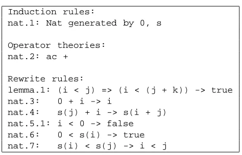
The display command enables users to view a set of objects. For example, if the display command is executed after the script in Figure 1 terminates, LP produces the output shown in Figure 2. Differences between what the user typed in Figure 1 and what LP displayed in Figure 2 reflect inferences performed by LP, as described in this and the next sections.

Optional arguments to the display command can be used to restrict the display to objects of specified types and with specified names. For example, if Figure 2 had been produced by the command display rewrite-rules nat (or display r nat, for short), it would have contained only the rewrite rules nat.3 to

nat.7.

In general, names begin with an identifier that consists of a sequence of letters, digits, and special characters such as underscores. LP is not sensitive to the case of letters in a name. Thus, Nat.1 and nat.1 refer to the same item. When displaying a name, LP uses the capitalization it found in the first occurrence of that name.

LP assigns new names of the form prefix.number (where prefix is “user” unless changed by the set name command, and where number increases each time a new name is required) to axioms introduced by the assert command, to critical-pair equations deduced in response to the critical-pairs and complete commands (see Sections 5.3 and 5.4), and to conjectures introduced by the prove command. LP assigns names of the form prefixCaseHyp.number, prefixInductHyp.number, etc., to case, induction, and other hypotheses it introduces during the proof of a conjecture. It assigns subnames of the form name.number to subgoals in a proof of a conjecture named name and to consequences deduced by instantiating (see Section 5.5) a fact named name or by applying a deduction rule (see Section 4.7).

Asterisks in name prefixes supplied as arguments to commands serve as patterns that match arbitrary sequences of characters in the prefix. For example, the command displayŁHyp causes LP to display all

facts whose name prefix ends with the letters Hyp.

Figure 14 in Section 7 provides details concerning these naming conventions.

3.5

Recording sessions

The command set log fileName causes LP to record all subsequent input and output in a file named

fileName.lplog (unless fileName contains a period, in which case LP does not supply the suffix .lplog).

Logging is ended by the unset log and quit commands.

The command set script fileName causes LP to record all subsequent user input in a file named

fileName.lpscr (unless fileName contains a period, in which case LP does not supply the suffix .lpscr). LP

annotates such a script file by commenting out illegal commands, by substituting the text of the executed file for an execute command, by marking the creation of subgoals and the completion of proofs, and by indenting the script file to reveal its proof structure. Scripting is ended by the unset script and quit commands.

Script files can be replayed using the execute command, and they can be edited before being replayed. Although a script file can be replayed directly using the command execute fileName.lpscr, it is generally advisable to rename the script file to fileName.lp and then replay it using the command execute fileName (lest a set script command cause LP to overwrite the command file being executed).

3.6

Settings

The set command can be used to control many aspects of LP’s behavior. Typing set alone causes LP to display a list of its current settings. Typing set followed by the name of a setting causes LP to display that setting and to prompt the user for a new value; responding with a carriage return leaves the setting unchanged. Typing set followed by the name of a setting and a value changes that setting. This section describes some elementary settings; Section 7.5 summarizes the others.

All settings have default values. The unset command can be used to reset a setting to its default value. The unset all command returns all settings to their default values.

set directory string

The directory is the name of the directory in which LP creates script (.lpscr), log (.lplog), and other output files. By default, directory is the name of the working directory from which LP was invoked.

set lp-path string

can be determined by typing the command version; it can be changed by invoking LP with the shell command lp d directoryName.

set page-modefonjoffg

When page-mode is off (the default setting), LP displays output continuously. When it is on, LP displays output a screenful at a time. At the end of each screenful, LP prompts the user with--More--to type a character indicating what to do next. The options are as follows:

Response Action

<space> display next screenful <return> display next line

<digit> display next<digit>lines d display next half screenful

u display continuously until next user interaction q display nothing until next user interaction ? display this menu

set prompt string

The prompt is the string that LP uses when prompting users to enter commands. The set prompt command allows users to change this prompt. If the new prompt begins or ends with a space, it should be enclosed within‘’marks, as in set prompt‘>> ’.

LP replaces the first exclamation mark (!) in the prompt, if any, by the number of the next command. LP numbers commands entered from the terminal by consecutive integers. It numbers commands obtained during execution of a command file by appending a period followed by consecutive integers to the command number for the execute command; thus command 5.2.3 is the third command in the file executed in response to the second command in the file executed in response to the fifth command typed by the user.

By default, prompt is‘LP!: ’ , which causes LP to issue prompts of the form “LP1: ”, “LP2: ”, : : :

set trace-level number

4

Defining theories

The basis for proofs in LP is a logical system consisting of a set of declared operators, the properties of which are axiomatized by equations, rewrite rules, operator theories, induction rules, and deduction rules (all expressed in a subset of multisorted first-order logic). Each kind of axiom has two semantics, a definitional semantics in first-order logic and an operational semantics that is sound with respect to the definitional semantics but not necessarily complete.

Sections 5 and 6 describe how axioms interact with LP’s proof techniques. Appendix B illustrates how they are used in a complete proof.

4.1

Declarations and identifiers

Identifiers for sorts, operators, and variables must be declared prior to use. Declarations (such as those in Figures 1 and 3) assign sorts to variables and signatures to operators. The symbol!(typed as->) separates the declaration for the domain of an operator (which is a list of sorts) from that of its range (which is a single sort). Constants (e.g., 0 and empty) are special cases of operators.

LP predefines the sort Bool, as well as the built-in operators true, false, if, not,D, & (and),j(or),) (implies, typed as=>), and,(if and only if, typed as<=>). It can also generate new variables, constants, and operators during the course of a session. The name of an LP-generated variable consists of the first letter of its sort, possibly followed by a number (e.g., n, n1 for sort Nat). The names of LP-generated constants end with the letter c, possibly followed by a number (e.g., xc or xc1). Users are not prevented from declaring such identifiers themselves, but may find it confusing to do so (or even unsound, if they mistakenly believe that they are declaring new constants).

Identifiers for sorts, variables, constants, and prefix operators are sequences of letters, digits, and special characters such as underscores ( ) and apostrophes (’). Identifiers for infix operators are sequences of characters drawn from an implementation-defined set of infix characters (e.g., “ !#$&*+-./<=>@\ˆ|˜”); the symbolsDDand!(i.e.,->) cannot be used for infix operators because LP reserves them for other uses. Identifiers for infix operators may also consist of a backslash (n) followed by a prefix identifier (e.g.,nin, which is printed in this guide as2by the conventions described in Section 3.1). The command help operator provides a precise description of LP’s lexicographical conventions.

LP automatically overloads the built-in operatorsDand if, once for each declared sort S, with signatures D:S;S!Bool and i f : Bool;S;S!S. Users can also overload identifiers. For example, the declarations

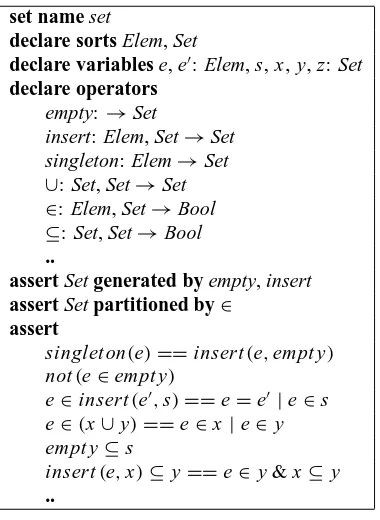
and axioms in Figure 3 can be used together with those in Figure 1 when reasoning about both natural numbers and sets. LP uses context to distinguish the variable s (of sort Set) from the operator s (with signature N at!N at). Users can overload other operators as well. For example, the commands

declare operators

[: Set, Elem!Set

[: Elem, Set!Set

.. assert

s[eDDinsert.e;s/ e[sDDinsert.e;s/

..

set name set

declare sorts Elem, Set

declare variables e, e0_{: Elem, s, x, y, z: Set} declare operators

empty:!Set

insert: Elem, Set!Set singleton: Elem!Set

[: Set, Set!Set

2: Elem, Set!Bool

: Set, Set!Bool

..

assert Set generated by empty, insert assert Set partitioned by2

assert

singlet on.e/DDinsert.e;empt y/ not.e2empt y/

e2insert.e0_;s/DDeDe0_je2s

e2.x[y/DDe2xje2 y empt ys

insert.e;x/yDDe2y & xy

..

Figure 3: Sample axiomatization for finite sets

restrictions on overloading identifiers is that users do not overload the built-in identifiers and that they do not declare an identifier both as a variable and as a constant of the same sort. The next section describes how to specify, when necessary, one of several possibly ambiguous overloadings of an operator.

The command display symbols causes LP to print a list of all declared identifiers.

4.2

Terms

A term in multisorted first-order logic consists of either a variable or of an operator and a sequence of terms, known as its arguments. The number and sorts of the arguments in a term must agree with the declaration for (some overloading of) the operator. The number of arguments is called the arity of the operator. An operator with arity 0 is called a constant. Infix operators are written between their arguments (e.g., iC j ), constants are written with no arguments (e.g, 0 or empty), and prefix operators

with nonzero arity are followed by a parenthesized list of arguments (e.g, s.i/or insert.e;x/).

LP uses a limited amount of precedence when parsing terms, but generally requires users to supply parentheses to specify the associativity of operators in terms with multiple infix operators. User-declared operators bind more tightly than the equality operator, which binds more tightly than the built-in boolean operators. Thus, LP parses the term.a<b & bDcCd/)a< .cCd/in the same way that it parses ..a<b/&.bD.cCd///).a< .cCd//. Unparenthesized sequences of infix operators at the same precedence level are permitted only in terms such as t1Ct2Ct3Ct4, which consist of a sequence of terms

aCbCc, but not p & qjr or aCb c.

In some cases, users must append qualifications to terms to clarify which of several overloadings of an identifier is meant. For example, given the declarations

declare operators a;b:!Nat, : Nat, Nat!Nat

declare operators a;b:!Set, : Set, Set!Set

it is ambiguous whether the term a b denotes the difference of two numbers or the difference of two

sets. To distinguish which of these two interpretations they intend, users must write either a:Nat b:Nat

or a:Set b:Set.4

4.3

Equations

LP is based on a subset of first-order logic in which equations play a prominent role. Figure 4, for example, contains LP commands that enter the usual first-order axioms for groups. Variables appearing in the axioms are implicitly universally quantified.

declare sort G

declare variables x;y;z: G

declare operators e: !G, i: G! G,Ł: G;G!G

assert

.xŁy/ŁzDDxŁ.yŁz/ eDDi.x/Łx

xDDeŁx

..

Figure 4: LP axiomatization of group theory

LP uses the logical symbolDDfor equality in an equation. This symbol is implicit in axioms such as 0<s.i/in Figure 1, which are shorthands for equations with right side true. LP bindsDDless tightly than the (overloaded) equality operatorD, so that, for example, e2insert.e0_;s/DDeDe0 _{je2s in}

Figure 3 can be written without more parentheses. It is parsed as .e2insert.e0;s//DD..eDe0/j.e2s//

The connectiveDD can appear only once in an equation, whereas D can appear many times. The definitional semantics makes no distinction betweenDDandD.

Equations can also be entered using the connective!instead ofDD. This constrains the way in which LP will orient them into rewrite rules (see Section 4.4), but does not alter their definitional semantics.

LP treats as inconsistent the equation t rue DD f alse and all equations of the form x DD t or not.xDt/DD t rue, where x is a variable and t is a term not containing x. Thus, LP is designed for

reasoning about models in which every sort has at least two elements.5 Inconsistencies can be used to associative, the term is parsed from left to right, for example, as..t1Ct2/Ct3/Ct4.)

4_{Release 2.2 of LP requires both a and b in these terms to be qualified, even though the sort of one determines the sort of} the other. For terms such as i=j , where i and j are unambiguous, but=is not, users can write.i=j/:Rational or.i=j/: Nat to disambiguate the term. Later releases of LP will do a better job of type inference.

establish subgoals in proofs of implications and in proofs by cases and contradiction. If they arise in other situations, they indicate flaws in the current logical system.

An equational theory is a theory (i.e., a set of facts) axiomatized by a set of equations. Equational theories can be characterized syntactically, as follows. The set of terms constructed from a set of variables and operators is called a free word algebra or term algebra. A set E of equations defines a congruence relation on a term algebra, this relation being the smallest one that contains the equations in E and that is closed under reflexivity, symmetry, transitivity, instantiation of free variables, and substitution of equals for equals. An equation t1DDt2is in the equational theory of E, or is an equational consequence of E,

if t1is congruent to t2.

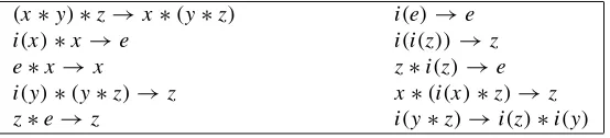
Figure 5 shows a sample informal proof that i.e/DDe is an equational consequence of the axioms for

groups in Figure 4.

Step Equation Justification

1. .xŁy/ŁzDDxŁ.yŁz/ Axiom

2. eDDi.x/Łx Axiom

3. xDDeŁx Axiom

4. .i.y/Ły/ŁzDDi.y/Ł.yŁz/ Replace x by i.y/in 1 5. eŁzDDi.y/Ł.yŁz/ Apply 2 to 4 (with y for x) 6. zDDi.y/Ł.yŁz/ Apply 3 to 5 (with z for x) 7. zDDi.i.z//Ł.i.z/Łz/ Replace y by i.z/in 6 8. zDDi.i.z//Łe Apply 2 to 7 (with z for x) 9. .i.i.e//Łe/Łi.e/DD Replace x by i.i.e//, y by e,

i.i.e//Ł.eŁi.e// z by i.e/in 1

10. eŁi.e/DDi.i.e//Ł.eŁi.e// Apply 8 to 9 (with e for z) 11. i.e/DDi.i.e//Łi.e/ Apply 3 to 10 (with e for x) 12. i.e/DDe Apply 2 to 11 (with i.e/for x)

Figure 5: Sample derivation from group axioms

4.4

Rewrite rules

Some of LP’s inference mechanisms work directly with equations. Most, however, require that equations be oriented into rewrite rules. Rewrite rules have the same logical meaning as equations, but behave differently operationally. A rewrite rule is an ordered pairhl;riof terms, usually written l ! r, such

that l is not a variable and every variable that occurs in r also occurs in l.6 _{A term-rewriting system, or a}

rewriting system for short, is a set of rewrite rules.

LP orients equations into rewrite rules and uses these rewrite rules to reduce terms to normal forms. For example, LP orients the equations asserted in Figure 1 into the rewrite rules displayed in Figure 2. The additional commands

declare operator 1:!Nat

assert 1DDs.0/ prove 1<1C1

1<1C1 by reducing it to t rue, as follows.

Term Derivation

1<1C1 Conjecture

s.0/ <s.0/Cs.0/ Apply 1!s.0/three times

s.0/ <s.0Cs.0// Apply nat.4 0<0Cs.0/ Apply nat.7 0<s.0/ Apply nat.3

true Apply nat.6

Note that rewrite rules nat.3 and nat.7 can be applied in either order.

To describe this process more precisely, we define a substitution¦to be a mapping from variables to terms such that¦.v/is identical tovfor all but a finite number of variables. The domain of a substitution is extended to terms in the usual way:¦.f.t1; : : : ;tn//is defined to be f.¦.t1/; : : : ; ¦.tn//. A substitution ¦matches a term t1to a term t2if¦.t1/is identical to t2.

Each rewriting system R defines a binary relation;R(rewrites or reduces directly to) on the set of all

terms. Operationally7_{, t}

;R u if there is some rewrite rule l ! r in R and some substitution¦ that

matches l to a subterm of t such that u is the result of replacing that subterm by¦.r/. The relation;

Ł

R (reduces or rewrites to) is the reflexive transitive closure of;R. Thus t ; Ł

R u if and only if there are terms t1; : : : ;tnsuch that t Dt1;R : : :;R tn Du. The relation;

C

R is the transitive irreflexive closure of;R. When R is clear from context, we write;for;R,;

Ł_for ;

Ł

R, and; C_for

; C R.

It is usually essential that R be terminating, in other words, that there be no infinite sequence

t1 ;R t2 ;R t3: : : of reductions. In general, it is undecidable whether a set of rewrite rules is

terminating. However, as discussed below, LP provides several mechanisms that automatically orient many sets of equations into terminating rewriting systems. For example, LP automatically orients the equations for groups in Figure 4 into the rewrite rules

.xŁy/Łz!xŁ.yŁz/ i.x/Łx!e

eŁx !x

It automatically reverses the left and right sides of the second and third equations, thus preventing nonterminating reduction sequences such as e ;i.e/Łe; i.e/Łi.e/Łe; : : :and e ; eŁe ;

eŁeŁe;: : :

8_{LP’s facilities for orienting equations into rewrite rules are discussed in Section 4.9.}

A term t is said to be irreducible if there is no term u such that t ;u. If t ; Ł

u and u is irreducible,

then u is a terminal or normal form of t . A term can have many different terminal forms. For example, both eŁz and i.y/Ł.yŁz/are normal forms of.i.y/Ły/Łz with respect to the rewrite rules for group

theory above.

Unless directed otherwise, LP keeps all rewrite rules and equations in normal form. If a rewrite rule or equation reduces to an identity, that is, to one in which the right and left sides have the same normal form, it is discarded.

If a term has only one normal form, that is called the canonical form of the term. A terminating rewriting

7_{Another characterization of}

;Ris as the smallest binary relation such that¦ .l/;R¦ .r/for every rewrite rule l!r in R

and every substitution¦, and such that f.t1; : : : ;ti; : : : ;tn/;R f.t1; : : : ;u; : : : ;tn/whenever ti;Ru.

system in which all terms have a canonical form is said to be convergent (cf. Appendix A).

If a rewriting system is convergent, its rewriting theory (that is, the equations that can be proved by reducing them to identities) is identical to its equational theory (that is, the equations that follow logically from the rewrite rules considered as equations). Unfortunately, most rewriting systems that arise in practice are not convergent. In these systems, the rewriting theory is a proper subset of the equational theory. For example, the equation i.e/ DDe is in the equational theory of the rewrite rules for group

theory above, as proved in Figure 5, but it is not in the rewriting theory (because it is irreducible and yet is not an identity).

The proof mechanisms discussed in Sections 5 and 6 compensate for the incompleteness that results when a system’s rewriting theory does not include all of its equational theory.

4.5

Operator theories

LP provides special mechanisms for handling some equations that cannot be oriented into terminating rewrite rules. The LP command assert acCin Figure 1 says thatCis associative and commutative. Logically, this assertion is merely an abbreviation for two equations:

xC.yCz/ DD .xCy/Cz xCy DD yCx

Operationally, it causes LP to use equational term-rewriting to match and unify terms (see Section 5.3) modulo associativity and commutativity. In equational term-rewriting, a substitution¦ matches t1to t2

modulo a set E of equations if¦.t1/DDt2is in the equational theory of E. For example, ifCis ac, the

rewrite rule aCb!c will reduce the term aCcCb to cCc.

Equational term-rewriting not only increases the number of theories that LP can reason about, but also reduces the number of axioms required to describe various theories, the number of reductions necessary to derive identities, and the need for certain kinds of user interaction, for example, case analysis. The main drawback is that equational term-rewriting can be much slower than conventional term-rewriting; associative-commutative matching, for example, is NP-hard, whereas conventional matching is linear. LP recognizes two nonempty operator theories: the associative-commutative theory (assert ac) and the commutative theory (assert commutative). The commutative theory is important because commutative axioms, such as x Cy DD yCx, cannot be oriented into terminating rewrite rules.

The associative-commutative theory is important because an equation describing associativity, such as .xCy/CzDDxC.yCz/, cannot be oriented into a terminating rule if commutative matching is used for the associative operator.

To facilitate matching terms involving ac or commutative operators, LP flattens the internal representation of terms by arranging the arguments to associative-commutative and commutative operators in a canonical order.9 The visible impact of this is that, when LP prints terms, the order in which arguments appear may be affected. For example, whenCis associative-commutative andDis commutative, LP will recognize.aCb/CcDd and dDbC.cCa/as having the same meaning, and it will print both as aCbCcDd. Flattening also explains why the display of nat.3 and nat.4 in Figure 2

differs from the original form of those equations in Figure 1.

4.6

Induction rules

LP allows users to axiomatize theories using induction rules, which are logically equivalent to infinite sets of first-order formulas. Induction rules increase the number of theories that can be axiomatized by finite sets of assertions. For example, none of the infinitely many facts not.i Ds.i//, not.i Ds.s.i///, : : : is an equational consequence of the equations in Figure 1.10_{But this infinite set of facts does follow}

when the equations are supplemented by the axiom

assert Nat generated by 0, s

The intuitive content of this axiom is that each element of sort Nat is either 0 or sn.0/, where n is a positive integer. This axiom is equivalent to the infinite set of first-order formulas11

.E[0]^.8i: N at/.E[i])E[s.i/]//).8j :N at/E[ j ]

where E is an arbitrary equation.12

As described in Section 6.3, LP uses induction rules to generate subgoals to be proved for the basis and induction steps in proofs by induction. The command

prove not.i Ds.i//by induction

directs LP to begin a proof of the conjecture not.i D s.i// by induction, in other words, to prove

not.0Ds.0//as the basis subgoal, and then to prove not.s.ic/ Ds.s.ic///as the induction subgoal using the induction hypothesis not.icDs.ic//, where ic is a new constant introduced by LP to formulate the induction hypothesis and subgoal.

Similary, the assertion Set generated by empty, insert in Figure 3 provides an induction rule for the sort

Set that is equivalent to the infinite set of axioms

.E[empt y]^.8e: Elem;s:Set/.E[s] )E[insert.e;s/]//).8s:Set/E[s]

Users can specify multiple induction rules for a single sort. For example, given the declarations in Figure 3, the LP commands

set name setInduction2

assert Set generated by empty, singleton,[

change the current name prefix and then assert that all objects of sort Set can be generated by taking unions of singleton and empty sets. Users can choose either induction rule when attempting to prove an equation by induction; for example,

prove xx by induction using setInduction2

As described in Section 6.11, users may use one induction rule to prove another. For example, a user might choose to prove rather than assert the rule setInduction2.

10_{For each n, there is a model of the equations that contains the natural numbers plus an additional n elements that form a cycle} under s and in which the relation a<b is always false when a and b are among these n elements.

11_{Because LP interprets induction axioms by sets of first-order formulas, these axioms do not rule out the existence of nonstandard} models, that is, of models that contain elements not of the form 0 or sn_{.0/, but with the same first-order properties as these elements.}

Interpreting induction axioms by single second-order sentences would rule out nonstandard models, but would not necessarily increase the number of theorems that can be proved (because complete systems of inference do not exist for second-order logic).

4.7

Deduction rules

LP uses deduction rules to deduce new equations from existing equations and rewrite rules. For example, the LP command

assert when iCj DDiCk yield j DDk

specifies a cancellation law for addition.13 Logically, this deduction rule has the same meaning as the equation iCj DiCk)j DkDDt rue, but there is an important operational difference: LP can apply

the deduction rule directly to the equation f.x/CcDDg.x/Cc to deduce the equation f.x/DDg.x/. Section 8 contains a discussion of the pragmatic ramifications of the differences between expressing axioms as deduction rules and expressing them as implications.

More powerful deduction rules allow explicit universal quantification of variables in their hypotheses. For example, the LP command

assert when.f orall e/e2xDDe2 y yield xDDy

defines a deduction rule equivalent to the universal-existential formula .8x;y:Set/[..8e: Elem/.e2x,e2y//)xDy]

of set extensionality. This deduction rule, which can also be asserted by the LP command assert S partitioned by 2, as was done in Figure 3, enables LP to deduce equations such as x DD x [x

automatically from equations such as e2 xDDe2.x[x/. (Section 5.5 shows another way to obtain this conclusion using the deduction rule.)

Deduction rules can have multiple hypotheses and/or multiple conclusions. For example, the transitivity of<can be formulated as a deduction rule with two hypotheses:

when i< j , j <k yield i<k

An example of a deduction rule with two conclusions is the &-splitting law:

when p & q yield p, q

where p and q have been declared as variables of sort Bool.

A deduction rule can be applied to an equation or a rewrite rule. An application succeeds if there is a substitution that matches the deduction rule’s first hypothesis to the equation or rewrite rule and that maps the variables in the forall clause to distinct variables14_{not appearing elsewhere}15_{in the matched}

equation or rewrite rule.

The result of applying a deduction rule with one hypothesis is the set of equations obtained by instantiating each of its conclusions by the substitution(s) that matched its hypothesis. LP substitutes fresh variables for variables that occur in the range of the matching substitution, but not in the hypothesis. For example, applying the deduction rule when P.x/yield Q.x;y/to P.f.y//produces the result Q.f.y/;y1/and not the weaker result Q.f.y/;y/.

The result of applying a deduction rule with more than one hypothesis is the set of deduction rules obtained by deleting the first hypothesis and instantiating the remainder of the deduction rule by the substitution(s) that matched it. For example, applying the deduction rule when x <y;y<z yield x<z

13_{Such cancellation laws generalize those used by Stickel [31] in reasoning about rings.}

14_{If the matched variables were not required to be distinct, then, for example, the deduction rule when (forall x;y) xŁz == yŁz}

yield zDD0 would apply to the equationwŁ1DDwŁ1 and yield the erroneous result 1DD0.

to the equation a<b yields the deduction rule when b<z yield a<z.

Deduction rules serve to increase LP’s logical power, to improve its performance, and to reduce the need for user interaction. Examples of deduction rules that serve the latter two purposes are the &-splitting law and the cancellation law for addition. The &-splitting law is so useful that it is built into LP to further improve performance.

LP automatically applies deduction rules to equations and rewrite rules whenever they are normalized. The sample proof in Appendix B illustrates the logical power of deduction rules, as well as the benefits of applying them automatically to additional hypotheses introduced in the course of a proof.

Like other facts in LP, deduction rules may be asserted as axioms or proved as theorems (cf. Section 6.10).

4.8

Built-in operators and axioms

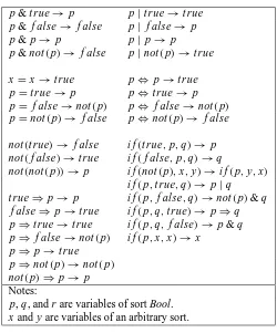
LP provides built-in rewrite rules (see Figure 6) to simplify terms involving the Boolean operators not , &,j,), and,, the overloaded equality operatorsD, and the overloaded conditional operators if.

p & t rue! p pjt rue!t rue p & f alse! f alse pj f alse! p p & p! p pj p! p

p & not.p/! f alse pjnot.p/!t rue xDx!t rue p, p!t rue pDt rue! p p,t rue! p pD f alse!not.p/ p, f alse !not.p/ pDnot.p/! f alse p,not.p/! f alse not.t rue/! f alse i f.t rue;p;q/! p not.f alse/!t rue i f.f alse;p;q/!q

not.not.p//! p i f.not.p/;x;y/!i f.p;y;x/ i f.p;t rue;q/! pjq t rue) p! p i f.p; f alse;q/!not.p/& q

f alse)p!t rue i f.p;q;t rue/! p)q p)t rue!t rue i f.p;q; f alse/! p & q p) f alse!not.p/ i f.p;x;x/!x

p) p!t rue p)not.p/!not.p/ not.p/)p! p

Notes:

p, q, and r are variables of sort Bool. x and y are variables of an arbitrary sort.

Figure 6: Rewrite rules built into LP

to be convergent and to yield all propositional identities) require exponential time and space [18, 32]. Furthermore, they can expand, rather than simplify, conjectures that do not reduce to identities. These are serious drawbacks, because when we are debugging specifications we often attempt to prove conjectures that are not true. So a complete set of rewrite rules for propositional logic is not built into LP. Instead, LP provides proof mechanisms that can be used to overcome incompleteness in a rewriting system, and it allows users to add any of the complete sets (which subsume the built-in rewrite rules) when they wish to use them.

LP also provides a built-in metarule for rewriting terms containing the conditional operator if. This metarule has the form

i f.t1;t2[t1];t3[t1]/!i f.t1;t2[t rue];t3[ f alse]/

and can be applied when t1occurs as a subterm of t2or t3. For example, LP uses this metarule to reduce

the term i f.p;p & q;pjr/to i f.p;q;r/.

LP treats &,j, and,as ac operators, and it treatsD, in all overloadings, as a commutative operator. Finally, LP provides the built-in deduction rules shown in Figure 7.16

lp not is true: when not.p/ yield pDD f alse lp not is false: when not.p/DD f alse yield p

lp and is true: when p & q yield p;q

lp or is false: when pjqDD f alse yield pDD f alse;qDD f alse lp iff is true: when p,q yield pDDq

lp equals is true: when xDy yield xDD y

Figure 7: Deduction rules built into LP

4.9

Orienting equations into rewrite rules

Ordinarily, LP automatically orients equations into rewrite rules without users having to enter explicit ordering commands. However, the set automatic-ordering off command causes LP to refrain from orienting equations until it receives an explicit order command.

LP provides three types of ordering mechanisms for orienting equations into rewrite rules. The command set ordering method can be used to select any of these mechanisms.

ž Two registered orderings (the dsmpos and noeq-dsmpos orderings), based on LP-suggested partial orderings of operators [6, 8], that guarantee termination of sets of rewrite rules when no commutative or associative-commutative operators are present.

ž A polynomial ordering, based on user-supplied polynomial interpretations of operators [1], that guarantees termination even when commutative or associative-commutative operators are present. Unfortunately, this powerful mechanism is difficult to use.

ž Three “brute-force” ordering procedures, which give users complete control over whether equations are oriented from left to right or from right to left. These provide no guarantees about termination.

Most users rely on LP’s registered orderings to order all equations; noeq-dsmpos is the default ordering. In striking contrast to the brute-force methods, they hardly ever cause difficulties by producing a nonterminating set of rewrite rules.

4.9.1 Registered orderings

LP’s registered orderings use information in a registry to orient equations. When no ac or commutative operators are involved, these orderings guarantee that the resulting rewrite rules terminate. There are two kinds of information in a registry: height information and status information.

Height information relates pairs of operators. If an operator f has greater height than another operator g, LP will attempt to orient equations containing f and g into rewrite rules that replace an occurrence

of f by one or more occurrences of g. For example, g.g.x//DD f.x/will be oriented into the rewrite rule f.x/!g.g.x//.

Status information assigns relative weights to the arguments of operators with arity greater than one. If

an operator h has left-to-right (right-to-left) status, more weight is assigned to h’s leftmost (rightmost) arguments. For example, if h has left-to-right status, h.f.x/;x/ DD h.x; f.x// will be oriented into the rule h.f.x/;x/ ! h.x; f.x//, whereas if h has right-to-left status it will be oriented into

h.x; f.x//!h.f.x/;x/. If an operator has multiset status, its arguments are given equal weight. If h has multiset status, the equation h.f.x/;x/DDh.x; f.x//cannot be oriented. LP automatically assigns multiset status to ac and commutative operators.

Figure 8 shows how the register command can be used to place information in the registry and how that information constrains the way in which equations are oriented. As discussed in Section 8, the register command can also be used to enhance performance.

Command Effect on ordering

register height f >g rewrite f to g

register height f Dg give f and g equal height

register height f ½g rule out g> f

register bottom f rewrite any non-bottom operator to f

register top f rewrite f to any non-top operator

register status right-to-left f assign more weight to f ’s right arguments register status left-to-right f assign more weight to f ’s left arguments register status multiset f assign equal weight to all arguments of f

Figure 8: LP commands for supplying ordering constraints

Information about the relative height of operators can be combined in a single command such as register height)> .&;j/ > t rue D f alse

which suggests that)be rewritten to either & orj, and that each of these be rewritten to true or false, which have the same height. The partial ordering on operators is transitively closed (so that)>t rue

is a consequence of this command). LP rejects register commands that do not represent a consistent addition to the registry, for example, commands that imply both f >g and g> f .

to be oriented from right to left. Furthermore, the noeq-dsmpos ordering does not generate suggestions assigning equal heights to two operators; as a result, it is faster, but less powerful than dsmpos.

Ordinarily, LP adds suggestions automatically to the registry when needed. These actions can be overridden by the command set automatic-registry off, which directs LP to ask the user to choose a suggestion to be added to the registry. For example, when asked to orient f.a;b/ DD f.b;a/with an empty registry, LP presents the user with the following suggestions for adding height and status information to the registry. Section 4.9.4 discusses how to respond to such suggestions.

Direction Suggestions --- ---1. -> a > b f(L) 2. -> b > a f(R) 3. <- b > a f(L) 4. <- a > b f(R)

Had the equation been entered as f.a;b/ ! f.b;a/, LP would have presented only the first two suggestions.

In addition to registering height and status information, a user may register operators as top or bottom operators. This does not immediately extend the height relation. When LP attempts to orient an equation that cannot be oriented with the current registry, but can be oriented by adding height relations that make non-top operators less than top operators, or non-bottom operators greater than bottom operators, LP will automatically extend the registry by adding such height relations, even if automatic-registry is off. Furthermore, registering an operator as bottom prevents LP from automatically extending the registry by making that operator greater than a non-bottom operator, and registering an operator as top prevents LP from automatically making that operator less than a non-top operator. However, unless it contradicts the current height relation, users may explicitly introduce relations in which bottom operators are greater than non-bottom ones and top operators are less than non-top ones.

The unregister command allows users to delete the entire registry, or to remove operators from the bottom or top of the registry, but not to remove height or status information in the registry (see Section 7.4).

4.9.2 Polynomial orderings

The polynomial ordering requires considerable user input. It is generally used only to experiment with termination proofs of small sets of rewrite rules, not to orient large sets of equations into rewrite rules.

The polynomial ordering is based on user-supplied interpretations of operators by sequences of polynomials [1]. The ordering extends these interpretations to terms by interpreting a variable by a sequence of identity polynomials and a compound term by the interpretation of its root operator applied to the interpretations of its arguments. One term is less than another in the polynomial ordering if its interpretation is lexicographically less than that of the second term (one polynomial is less than another if its value is less than that of the other for all sufficiently large values of its variables).

The command set ordering polynomial length sets the current ordering to a polynomial ordering based on sequences containing length polynomials; if no length is specified, it is assumed to be 1.

If the sequence of polynomials associated with an operator is longer than the length of the current polynomial ordering, the extra polynomials are ignored. If it is shorter, it is extended by replicating its last element.

The commands in Figure 9, if issued before asserting the axioms in Figure 1, cause LP to use the polynomial ordering to prove that set of rewrite rules shown in Figure 2 terminates. For example, they cause LP to orient s.i/Cj DD s.iC j/from left to right, because the polynomial interpretation .iC2/Ł j of the left side dominates the interpretation iŁ jC2 of the right side when j is sufficiently large, for example, when j >1. The noeq-dsmpos ordering produces the same set of rewrite rules as this polynomial ordering, but does not guarantee that they terminate, becauseCis ac.

set ordering polynomial

register polynomial 0 2

register polynomial s xC2

register polynomial C xŁy

register polynomial < xŁy

Figure 9: Sample polynomial interpretation

4.9.3 Brute-force orderings

These orderings provide no guarantee about termination.

The manual ordering causes LP to ask the user how to orient each equation. The user is allowed to choose either orientation, provided it results in a valid rewrite rule, that is, provided that the left side of the resulting rewrite rule does not consist of a variable and that the right side does not introduce a variable not present in the left side.

The left-to-right ordering causes LP to orient equations into rewrite rules from left to right, provided the results are valid rewrite rules. The either-way ordering behaves like the left-to-right ordering, except that it orients an equation into a rewrite rule from right to left if that is possible and left to right is not.

4.9.4 Interacting with the ordering procedures

When automatic-ordering is off, users must issue explicit order commands to cause LP to orient equations into rewrite rules. When automatic-registry is off, LP will prompt users to confirm any extensions to the registry when a registered ordering is in use, or to select an action for an equation LP is unable to orient. When presented with a prompt like

The following sets of suggestions will allow the equation to be ordered:

Direction Suggestions --- ---1. -> a > b 2. <- b > a

What do you want to do with the equation?

Enter one of the following, or type <ret> to exit. accept[1..2] kill postpone

divide left-to-right right-to-left interrupt ordering suggestions

of possible responses, which have the following effects.

ž accept (or a number in the indicated range): confirms the first (or the selected) extension to the registry.

If this action is missing from the menu, no extension to the registry will orient the equation.

ž divide: causes LP to add two new equations that imply the original equation. This action is useful

when an equation such as x=xDD y=y cannot be oriented because each side contains a variable not

in the other side. If the user elects to divide this equation, LP will ask the user to supply a name for a new operator, for example, e; it will then declare the operator and assert two equations, x=xDDe

and y=yDDe, both of which can be oriented (by making=higher than e) and which normalize the original equation to an identity.

ž interrupt: interrupts the ordering process and returns LP to command level.

ž kill: deletes the problematic equation from the system. This should be used with caution, since it may

change the theory associated with the current logical system.

ž left-to-right: orients the equation from left-to-right without extending the registry. Doing this removes

any guarantee of termination.

ž ordering: displays the current registry (as does display ordering at the command level) and prompts

the user for another response.

ž postpone: defers the attempt to orient this equation. Whenever another equation is successfully

oriented, all postponed equations are re-examined, since they may have been normalized into something more tractable.

ž right-to-left: orients the equation from right-to-left without extending the registry. Doing this removes

any guarantee of termination.

ž suggestions: redisplays the LP-generated suggestions for extending the registry and prompts the user