Computer Science Dissertations Department of Computer Science
Fall 12-14-2010
Dynamic Data Driven Application System for
Wildfire Spread Simulation
Feng Gu
Georgia State University
Follow this and additional works at:https://scholarworks.gsu.edu/cs_diss
Part of theComputer Sciences Commons
This Dissertation is brought to you for free and open access by the Department of Computer Science at ScholarWorks @ Georgia State University. It has been accepted for inclusion in Computer Science Dissertations by an authorized administrator of ScholarWorks @ Georgia State University. For
more information, please [email protected].
Recommended Citation
DYNAMIC DATA DRIVEN APPLICATION SYSTEM FOR WILDFIRE SPREAD SIMULATION
by
FENG GU
Under the Direction of Xiaolin Hu
ABSTRACT
Wildfires have significant impact on both ecosystems and human society. To effectively manage
wildfires, simulation models are used to study and predict wildfire spread. The accuracy of
wildfire spread simulations depends on many factors, including GIS data, fuel data, weather
data, and high-fidelity wildfire behavior models. Unfortunately, due to the dynamic and
complex nature of wildfire, it is impractical to obtain all these data with no error. Therefore,
predictions from the simulation model will be different from what it is in a real wildfire.
Without assimilating data from the real wildfire and dynamically adjusting the simulation, the
difference between the simulation and the real wildfire is very likely to continuously grow. With
the development of sensor technologies and the advance of computer infrastructure, dynamic
data driven application systems (DDDAS) have become an active research area in recent years.
In a DDDAS, data obtained from wireless sensors is fed into the simulation model to make
predictions of the real system. This dynamic input is treated as the measurement to evaluate
the output and adjust the states of the model, thus to improve simulation results. To improve
the accuracy of wildfire spread simulations, we apply the concept of DDDAS to wildfire spread
The assimilation system relates the system model and the observation data of the true state,
and uses analysis approaches to obtain state estimations. We employ Sequential Monte Carlo
(SMC) methods (also called particle filters) to carry out data assimilation in this work. Based on
the structure of DDDAS, this dissertation presents the data assimilation system and data
assimilation results in wildfire spread simulations. We carry out sensitivity analysis for different
densities, frequencies, and qualities of sensor data, and quantify the effectiveness of SMC
methods based on different measurement metrics. Furthermore, to improve simulation results,
the image-morphing technique is introduced into the DDDAS for wildfire spread simulation.
INDEX WORDS: Wildfire spread, Modeling, Simulation, DEVS, DDDAS, Sequential Monte Carlo
DYNAMIC DATA DRIVEN APPLICATION SYSTEM FOR WILDFIRE SPREAD SIMULATION
by
FENG GU
A Dissertation Submitted in Partial Fulfillment of the Requirement for the Degree of
Doctor of Philosophy
In the College of Arts and Sciences
Georgia State University
Copyright by
Feng Gu
DYNAMIC DATA DRIVEN APPLICATION SYSTEM FOR WILDFIRE SPREAD SIMULATION
by
Feng Gu
Committee Chair: Xiaolin Hu
Committee: Rajshekhar Sunderraman
Saeid Belkasim
Jiawei Liu
Electronic Version Approved:
Office of Graduate Studies
College of Arts and Sciences
Georgia State University
ACKNOWLEDGEMENTS
First of all, I thank my advisor Dr. Xiaolin Hu for his supervision in the past four years. He is an
excellent researcher, full of creativity and innovative. He taught me how to express my ideas. He
guided me to approach a research problem and persistently accomplish the goal. I was deeply
impressed by his enthusiasm for research. Besides my advisor, I would like to thank my
dissertation committee, Dr. Rajshekhar Sunderramn, Dr. Saeid Belkasim, and Dr. Jiawei Liu, for
their insightful comments. During the course of my dissertation, I was supported in part by
grants CNS-0841170 and CNS-0941432 from the National Science Foundation.
Also, I thank my family, my father Jinxue Gu, my mother Xiumei Wen, for their endless love
and support, my sisters Shufen Gu and Shufang Gu, for their believing in me. I never feel my
mother has left, giving me bravery, courage, and strength. Last but not least, I express my thanks
to Yinting Xu, for his encouraging and trusting me.
TABLE OF CONTENTS
ACKNOWLEDGEMENTS ... iv
LIST OF TABLES ... viii
LIST OF FIGURES ... ix
CHAPTER 1 INTRODUCTION ...1
1.1 Problem statement ...1
1.2 Structure of DDDAS ...2
1.3 The organization of the work ...5
CHAPTER 2 RELATED WORK ...6
2.1 Applications and algorithms of data assimilation ...6
2.1.1 Applications of data assimilation ...6
2.1.2 Algorithms of data assimilation ...7
2.2 Wildfire spread modeling ...10
2.3 Sequential Monte Carlo methods and their applications ...11
2.3.1 Overview of sequential Monte Carlo methods ...11
2.3.2 Applications of sequential Monte Carlo methods ...13
2.4 Applications of dynamic data driven application systems ...14
CHAPTER 3 WILDFIRE SPREAD MODEL OF DEVS-FIRE ...17
3.1 Concepts of DEVS ...17
3.1.1 Framework of M&S ...17
3.1.2 DEVS formalism ...18
3.1.3 Applications of DEVS ...19
3.2 Wildfire spread model using DEVS —DEVS-FIRE ...20
3.2.1 System architecture of DEVS-FIRE...20
3.2.3 Specification of DEVS-FIRE ...24
3.2.4 Interface of DEVS-FIRE ...25
CHAPTER 4 MEASUREMENT MODEL ...27
4.1 Computation of temperatures ...28
4.2 Example of the measurement model ...30
4.3 Sensor deployment schema ...31
CHAPTER 5 DATA ASSIMILATION IN DEVS-FIRE SIMULATION ...33
5.1 Problem formulation ...33
5.2 Data assimilation using SMC methods ...34
5.2.1 Sampling using DEVS-FIRE simulation ...38
5.2.2 Weight computation ...41
5.2.3 Resampling algorithm ...43
5.3 Software architecture ...45
CHAPTER 6 EXPERIMENTAL RESULTS ...48
6.1 Experimental methods and designs ...48
6.2 Experimental results ...50
6.2.1 Wind speed ...50
6.2.2 Wind direction ...54
CHAPTER 7 SENSITIVITY ANALYSIS ...57
7.1 Errors between the real system and the simulation system ...57
7.2 Sensor density ...62
7.3 Frequency of sensor data...66
7.4 Quality of sensor data ...68
CHAPTER 8 MEASUREMENT ANALYSIS ...72
8.1.1 Convergence metrics ...72
8.1.2 Degeneracy metrics ...73
8.1.3 Sample impoverishment ...74
8.2 Analysis of SMC methods in DEVS-FIRE...75
8.2.1 Convergence analysis ...75
8.2.2 Degeneracy analysis ...81
8.2.3 Sample impoverishment analysis ...81
CHAPTER 9 APPLYING IMAGE MORPHING TO DDDAS ...84
9.1 Basics of image morphing ...84
9.2 Applying image morphing in DEVS-FIRE ...85
9.3 Improvement of SMC methods of DEVS-FIRE ...86
CHAPTER 10 VALIDATION OF DEVS-FIRE ...89
10.1 Experimental design ...90
10.2 The fuels and the wind factors ...92
10.3 The slope and the aspect factors ...96
10.4 Non-uniform fuel/slope/aspect ...99
10.5 GIS data and varying wind condition ...101
CHAPTER 11 DISCUSSIONS AND FUTURE WORK ...104
11.1 Discussions ...104
11.2 Conclusions and future work ...106
REFERENCES ...108
LIST OF TABLES
Table 6.1 Experimental sets of wind factor 49
Table 7.1 Experimental sets of different errors 57
Table 10.1 Input sets 91
Table 10.2 Hypothesis test results 99
Table 10.3 GIS data with non-uniform fuel/slope/aspect 101
LIST OF FIGURES
Figure 1.1 Structure of the dynamic data driven system for wildfire spread simulation 4
Figure 3.1 Framework of M&S 17
Figure 3.2 Structure of DEVS-FIRE 21
Figure 3.3 State transitions of forest cells 23
Figure 3.4 Decomposition schema of DEVS-FIRE 23
Figure 3.5 Graphical output of fire spread in DEVS-FIRE 26
Figure 4.1 Real time data collection 27
Figure 4.2 Relationship between the distance and the temperature 29
Figure 4.3 Example of the measurement model 30
Figure 4.4 Temperature maps of the measurement model 32
Figure 5.1 Data assimilation based on SMC methods 36
Figure 5.2 Fire front estimation by assimilating ground temperature sensor data 38
Figure 5.3 Fire fronts with random noises 41
Figure 5.4 Adjusted weight computation (a=0.3) 43
Figure 5.5 Multinomial resampling 45
Figure 5.6 Computational architecture 46
Figure 6.1 Real fireand simulated fires for case 1 and case 2 51
Figure 6.2 Comparisons of real fire, simulated fires, and filtered fires for case 1 and case 2 52
Figure 6.3 Perimeters and areas of real fire, simulated fires, and filtered fires for case 1 and case 2 53
Figure 6.4 Symmetric set differences for case 1 and case 2 54
Figure 6.6 Comparisons of real fire, simulated fires, and filtered fires
for case 3 and case 4 55
Figure 6.7 Perimeters and areas of real fire, simulated fires, and filtered fires for case 3 and case 4 56
Figure 6.8 Symmetric set differences for case 3 and case 4 56
Figure 7.1 Simulated fires for case 5~8 58
Figure 7.2 Comparisons of real fire, simulated fires, and filtered fires for case 5 ~ 8 59
Figure 7.3 Relationship between the wind conditions and the perimeters and areas of real fire, simulated fires, and filtered fires 61
Figure 7.4 Relationship between symmetric set differences and wind conditions 62
Figure 7.5 Fire spreads with various sensor deployment schemas 64
Figure 7.6 Fire perimeters and areas of real fire, simulated fire, and filtered fires with sensor densities 65
Figure 7.7 Decreased symmetric set differences (SSD) with sensor densities 66
Figure 7.8 Fire spreads with various data frequencies 67
Figure 7.9 Perimeters and areas of real fire, simulated fire, and filtered fires with various data frequencies 68
Figure 7.10 Decreased symmetric set differences (SSD) with sensor data frequencies 68
Figure 7.11 Fire spreads with various sensor data errors 70
Figure 7.12 Perimeters and areas of real fire, simulated fire, and filtered fires with different sensor data errors 71
Figure 7.13 Decreased symmetric set difference (SSD) with sensor data errors 71
Figure 8.2 Convergence of the first case 76
Figure 8.3 Convergence of the second case 76
Figure 8.4 Convergence procedure of the first case 80
Figure 8.5 Exceedence ratios of case 1 and case 81
Figure 8.6 Sample impoverishment analysis for case 1 82
Figure 8.7 Sample impoverishment analysis for case 83
Figure 9.1 Image morphing in DEVS-FIRE 86
Figure 9.2 Real fire, simulated fire, and filtered fire after using image morphing in SMC methods for case 5 in Chapter 7 88
Figure 10.1 Uniform cases without aspect and slope 93
Figure 10.2 Uniform cases without aspect and slope 95
Figure 10.3 Uniform cases with different wind speeds 95
Figure 10.4 Uniform cases with aspect and slope 97
Figure 10.5 Data with different aspects 97
Figure 10.6 Data with different slopes 98
Figure 10.7 Non-uniform cases 100
CHAPTER 1 INTRODUCTION
1.1 Problem statement
Wildfires have significant impact on both the ecosystems and human society. The effects on
ecological systems include burning local plants, reducing species diversity due to the emission of
carbon dioxide, destroying organic nutrients to cause flash floods, and leading to climate changes
by releasing carbon into atmosphere (Keeley 1995; Lindsey 2008; Kennard 2008; Running
2008). Wildfires also cause massive losses of natural forest resources, endangered species,
properties, and even human lives. It is estimated that more than 11,000 communities close to
federal land are subject to threats from wildfires in the US (Rey 2004). In the 2007 wildfire
season, over 85,500 fires across the whole US burned more than 9.3 million acres of land. It cost
1.8 billion dollars in effort to fight wildfires and a potential 2.5 billion dollars in insured loss in
California alone (Grossi 2007). To effectively manage wildfires, simulation models are used to
study and predict wildfire spread. Over the years, several major wildfire spread simulation
models have been developed, including FARSITE (Finney 1998), BehavePlus (Andrews et al.
2005), DEVS-FIRE (Ntaimo et al. 2008), and HFire (Morais 2001).
The accuracy of wildfire spread simulations depends on many factors, including GIS data,
fuel data, weather data, and high fidelity wildfire behavior models. Unfortunately, due to the
dynamic and complex nature of wildfire, it is impractical to obtain all these data with no error.
For example, the weather data used in the simulation is typically obtained from local weather
stations in a time-based manner (e.g., every 10 minutes). Before the next data arrives, the
weather is considered unchanged in the simulation model. This is different from the reality
where the real weather constantly changes (e.g., due to the interactions between wildfires and the
resolutions. Besides data errors, the wildfire behavior model introduces errors too because of its
computational abstraction. Due to these errors, the predictions from the simulation model will be
different from what it is in a real wildfire. Without assimilating data from the real wildfire and
dynamically adjusting the simulation, the difference between the simulation and the real wildfire
is very likely to continuously grow.
With the development of sensors technologies and the advance of computer infrastructure, dynamic data driven application systems (DDDAS) become an active research area in recent
years. In a DDDAS system, the data obtained from wireless sensors is fed into the simulation
model to make predictions of the real systems. This dynamic input is treated as the measurement
to evaluate the output and adjust states of the model. Based on these measurements, we can
evaluate, choose, or analyze the system states utilizing statistical tools, data processing, and
numeric or non-numeric techniques to improve the simulation results. To improve the accuracy
of wildfire spread simulations, we also introduce the concept of DDDAS, which dynamically
assimilates sensor data from real wildfires into the model to produce a time sequence of
assimilated states. The assimilation systems map data between the model and the observation
data and evaluate the system states to obtain the state estimations.
1.2 Structure of DDDAS
In a typical DDDAS, there exist three major components, including the application (the
model system), the measurement model, and data assimilation methods. Therefore, it generates a
wealth of new challenges for applications, algorithms, performances, and measurement
approaches. For the wildfire spread simulation, the DEVS-FIRE model is developed as an
integrated environment for surface wildfire spread and containment, built on Discrete Event
model, the real time data on-site is considered to be introduced to improve the simulation results.
Therefore, the measurement model, which is used to couple the application model and real time
data, should be developed, thus to compare the application model’s output with the real data, and
further estimate the real state of the system.
To effectively utilize the real time data in the system model and the measurement model,
data assimilation methods that assimilate sensor data from real wildfires are needed. Data
assimilation is an analysis technique, in which the observed data is accumulated into the model
to produce a time sequence of assimilated states (Bouttier and Courtier 1999). Given a state
space model of a system, related approaches are designed to estimate a system state from the
observation data, including the simple analysis method and the statistical approach. The simple
analysis method simply and directly utilizes the observation data for the state estimation of the
system without considering all kinds of errors. Instead, the statistical approach assumes the
estimations from the system model and the observations have errors and all the error are
unknown but known distributed. Using these statistical tools, we try to find the estimation of the
state given the observation data.
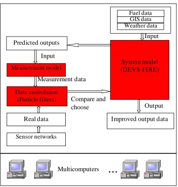
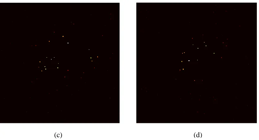
As described above, the structure of DDDAS for wildfire spread simulation is displayed in
Figure 1.1. From Figure 1.1, we can see that the key components of the dynamic data driven
system for wildfire spread model are the system model, the measurement model, and the data
assimilation system. Basically, we use the physical model to predict the fire spread if there are
the input sets including fuel data, GIS data, and weather data available. This static wildfire
spread model is the basis of fire prediction. The measurement model is the connection between
the wildfire spread model and the real time data. Fire sensors are deployed in the fire space and
the data to the data assimilation system, which is compared with the real data from sensor
networks. Consequently, the data assimilation system chooses the fire states as the inputs of
DEVS-FIRE, continuing to execute the system model to predict the next fire state. Because we
consider the uncertainty of fire states in the system, which will introduce a lot of computations,
the whole system is constructed on the multicomputer environment, in which multiple
computational units run the simulations in parallel to improve the performance.
System model (DEVS-FIRE)
Fuel data GIS data Weather data
Improved output data Predicted outputs
Real data Measurement model
Sensor networks Data assimilation
(Particle filters)
Multicomputers
…
Input
Output Compare and
choose Input
[image:18.612.128.488.259.637.2]Measurement data
1.3 The Organization of the work
Based on the structure of DDDAS, the work will construct the entire system consisting of
all the components, which will be explained later. Chapter 2 introduces the related work of data
assimilation, wildfire spread models, sequential Monte Carlo methods, and dynamic data driven
application systems. Chapter 3 describes DEVS-FIRE, the wildfire spread model we use in this
work. Chapter 4 explains the measurement model, which maps between the system model and
real time data. In Chapter 5, the data assimilation system is presented. Using identical twin
methods, we design corresponding experiments to test the DDDAS for wildfire spread
simulation in Chapter 6. Also, sensitivity analysis is done based on the experimental results in
Chapter 7, including errors between the real system and the simulated system, the density of
deployed sensors, the frequency of sensor data, and the quality of sensor data. To evaluate the
data assimilation method, related measurement metrics are introduced in Chapter 8, thus to
provide guidelines to develop more advanced algorithms. Additionally, image morphing is
borrowed to DDDAS to improve the simulation results in Chapter 9. Chapter 10 provides the
CHAPTER 2 RELATED WORK
2.1 Applications and algorithms of data assimilation
2.1.1 Applications of data assimilation
Data assimilation is used in many different fields, such as geosciences, weather forecasting,
hydrology, and other environmental systems. The purpose of data assimilation is to use
observation information to improve state estimation of a system under study. It tries to find the
solutions by minimizing the errors between the real system and the models. The optimal
interoperation analysis techniques are widely used in data assimilation, such as
three-dimensional variational analysis (3D-VAR) and four-three-dimensional variational assimilation
(VAR). Although both of them minimize the cost function to obtain optimal estimations,
4D-VAR incorporates a prediction model to compare the model state and the observations at
different time steps. The work of Bei et al. (2008) proposed a data assimilation system to
improve ozone simulations in Mexico City basin using 3D-VAR that generated the optimal
estimate of the true atmospheric state during the analysis time. Wilkin et al. (2008) used satellite
remotely sensed observations to the regional ocean modeling system in ocean analysis and
prediction, in which 4D-VAR was the primary analysis technique. It combined observations and
modeling to produce an optimal estimation of the real ocean state. Kalman filter (Kailath et al.
2000) is an analysis technique that estimates the state of a dynamic system with observations
represented by a linear state space model. For applications with non-linear behaviors, the
classical Kalman filter needs to be extended. Antoniou et al. (2007) studied three extensions of
Kalman filter including extended Kalman filter, limited extended Kalman filter, and unscented
In the wildfire spread simulation, less research exists in data assimilation. In the limited
work that we are aware of, Bradley (2007) proposed an approach to estimate forest fires based on
sequential Monte Carlo methods from video images. In this work, a blurring function was used
to add uncertainty to the images, and the information from miniature air vehicles was used as the
measurement data to estimate fire poses. No wildfire spread simulation model was used in this
work. Another group of work (Mandel et al. 2004; Mandel et al. 2009; Douglas et al. 2006; Coen
et al. 2007) used data assimilation to investigate fire behaviors of wildfire spread models. Their
work was built on a reaction-diffusion-convection partial differential equation model and used
ensemble Kalman filter as the estimation method. In their work, the real time data was
assimilated into the fire model to estimate the temperature of each cell. Our previous work (Gu
and Hu 2008; Gu et al. 2009; Yan et al. 2009) explored applications of sequential Monte Carlo
methods to state estimation in wildfire spread simulation using a discrete event simulation
model. Preliminary results showed that sequential Monte Carlo methods were promising
techniques for supporting data assimilation in wildfire spread simulations.
2.1.2 Algorithms of data assimilation
The methods of data assimilation include the simple analysis approach and the statistical
approach. The simple analysis method considers the observation as the ―truth‖, and directly and
simply uses the observation data. The state of the model is set to the observation values close to
available observations and to an arbitrary state otherwise. Cressman analysis is one of simple
analysis methods. In Cressman analysis, the analysis is generated by interpolating between the
background (the previous estimate of the model state) and the observations, in the vicinity of
each observation value. The simple analysis method is the basic tool because of its simplicity.
problems (the existing errors of background and observations) and obtain quality estimations,
better methods to combine uncertainty are needed.
In the statistical approach, we try to use all the information, but don’t completely trust
them. We can find a strategy to minimize the average of the differences between the analysis and
the truth. In this sense, the analysis can be seen as the optimization problem. All the related
errors are assumed to be unknown and have known statistical properties. There are two main
ways to define the statistical analysis problem. The first one is to assume that the background
covariance and error covariance are known, and derive the analysis equations according to the
constraint that total analysis error variances are minimum. In the second approach, we hold the
assumption that the probability density functions of the background and observation errors are
Gaussian, thus to derive the analysis equations by obtaining the state with maximum probability.
Both of the approaches lead to kinds of algorithms, directly determining the analysis gain matrix
and/or minimizing a quadric cost function, although their numerical properties greatly differ.
The optimal interpolation (OI) is a technique to simply and directly compute the gain matrix
using matrix operations. The basic assumption of OI is that for each model variable, only a few
observations are important. This will raise the question how to decide the used observations for
the model variables. Two common selection schemas are used including pointwise selection and
box selection. In pointwise selection, each analysis point is only sensitive to observations within
a small range and two neighboring points have different observation sets. For box selection, all
points in an analysis box are located in a larger selection box and two neighboring analysis boxes
have almost the same observations. The advantages of OI include easy implementation and small
observations are used in different parts of the model state. For the small and large scale analysis,
it possibly leads to inconsistency.
Instead of computing gain matrix, three-dimensional variational analysis (3D-VAR) tries to
find an approximate solution to the equivalent minimization problem defined by the cost
function, evaluating the cost function and its gradients several times. 3D-VAR is popularly used
because of its simplicity and supporting complex observation operators. Also, it also accepts the
external constraints. Four-dimensional analysis (4D-VAR) is a simple generalization of 3D-VAR,
in which observations are distributed in time. In 4D-VAR, the observation operators include a
forecast model used to compare the model state and the observations at the appropriate time
steps. Comparing with 3D-VAR, 4D-VAR works only if the model is perfect.
Kalman filter and its extended version (extended Kalman filter) are developments of least
squares analysis in the sequential data assimilation. The extended Kalman filter doesn’t need the
linear model operator and/or observation operator. Their inputs include the definitions of the
model operator and the observation operator, the initial conditions, and the sequences of
observations. Kalman filter is done in a recursive manner. The estimates from the previous step
and the current observation are used for the current state estimation. Two basic steps are
involved in Kalman filter including predict and update. The predict step uses the estimates from
the last step to produce the current state. In the update stage, the current a prior prediction is
combined by the observation, thus to refine the current estimate to produce a posterior prediction.
Kalman filter has many common features with 4D-VAR. In essential, if the model is perfect with
the same time interval and input data, 4D-VAR analysis at the last time step is equal to that of
Kalman filter at the same time step. They also differ in many aspects: (1) 4D-VAR is
and is not sequential; (3) 4D-VAR runs for a finite time interval, whereas Kalman filter can
implement forever if the observations at the next step are available; (4) 4D-VAR must meet the
requirements that the model is perfect. Ensemble Kalman filter is from a version of Kalman filter
with large number of variables. It is related to sequential Monte Carlo methods (particle filters)
discussed in the next sections and adopted in this work. However, ensemble Kalman filter
assume that all probability functions involved are Gaussian, and it is more efficient than
sequential Monte Carlo methods. Note that the details of the most of algorithms above can be
found in (Bouttier and Courtier 1999).
2.2 Wildfire spread modeling
Simulations of wildfire can be categorized into two approaches, the physical approach and
the empirical approach. The physical approach considers fire spread as heat transfer between
burning and unburned fuel using partial differential equations to solve for filtered fire spread (see
(Douglas et al. 2006; Linn et al. 2002; Pastor et al. 2003; Weber 1991)). The empirical approach
relies on statistical correlations between variables known to influence fire spread with field observations of rates of spread. A widely used empirical fire behavior model is Rothermel’s
model (Rothermel 1972). Several major wildfire simulation systems have been developed to date,
including FARSITE (Finney 1998), BehavePlus (Andrews et al. 2005), and HFire (Morais 2001). These systems use Rothermel’s fire behavior model to compute the rate of fire spread, and
determine the fire size according to an elliptical shape. They are raster-based spatially explicit
models, and use a discrete time approach for simulating the wildfire growth. Many complex
simulation models allow the wildfire to feed back upon the atmosphere. FIRETEC, a wildfire
behavior model developed at Los Alamos National Laboratory, explored the interactions
discrete event wildfire simulation model called DEVS-FIRE (Ntaimo et al. 2008; Hu et al. 2010) that used Rothermel’s fire behavior model too. The DEVS-FIRE model is described in more
details in Chapter 3.
2.3 Sequential Monte Carlo methods and their applications
2.3.1 Overview of sequential Monte Carlo methods
Sequential Monte Carlo (SMC) methods are sample-based methods that use Bayesian
inference and stochastic sampling techniques to recursively estimate the state of dynamic
systems from some given observations. A dynamic system is formulated as discrete dynamic
state-space model, which is composed of the system model of equation (2.1) and the
measurement model of equation (2.2) (Jazwinski 1970) as shown below. In the equations, t is
time step, st and mt are the state variable and the measurement variable respectively, the
functions of f and g define the evolutions of the state variable and the measurement variable, and
vt and wt are two independent random variables to generate the state noise and the measurement
noise.
st1 f(st,t)vt. (2.1)
mt g(st,t)wt. (2.2)
For state estimation, one needs to seek estimates of st based on the set of all measurements
}. ,..., 2 , 1 , { :
1 m i t
m t i In Bayesian filtering, both the state and the measurement variables are
stochastic variables. Assuming the probability density p(st1|m1:t1) at time step t-1 is available,
the prior probability density function of the state at time step t can be obtained using the system
model as shown in equation (2.3), where p(st |st1) is the system model. If the measurement at
theorem as shown in equation (2.4). In equation (2.4), p(mt |st) can be obtained by the
measurement model, and p(mt |m1:t1) is a normalizing constant that can be computed by
equation (2.5) according to Bayes theorem and Markov property. Equation (2.3) and equation
(2.4) form the foundation to recursively predict the prior probability density function, and update
it to the needed posterior probability density function of the current state.
p(st m1:t1) p(st st1)p(st1m1:t1)dst1. (2.3)
) ( ) ( ) ( ) ( 1 : 1 1 : 1 : 1 t t t t t t t t m m p m s p s m p m s
p . (2.4)
p(mt m1:t1)p(mt st)p(st m1:t1)dst. (2.5)
Because it is difficult to solve the multidimensional integrals, many approximation algorithms
are proposed, among which SMC methods are described below.
SMC methods approximate the posterior probability density function p(st |m1:t) by a set of
samples and their corresponding weights. An important concept in SMC methods is the principle
of sequential importance sampling (SIS). In SIS, the posterior probability function is
approximated by equation (2.6), where st(i) and wtt(i) are particle i at time step t and its
normalized weight, and δ is the delta function. The weights are defined in equation (2.7), where
) , |
(st(i) st(i)1 mt
q is the importance density, which can be easily generated.
( | ) () ( ()) 1 : 1 i t t i t N i t
t m wt s s
s
p
. (2.6)
) , | ( ) | ( ) | ( 1 ) ( ) ( 1 ) ( ) ( ) ( 1 ) ( t i t i t i t i t i t t i t i t m s s q s s p s m p wt wt
However, sequential importance sampling has the limitation that the entire process relies on the
initially generated samples. To improve the algorithm, a resampling step is added by using
replicated particles in proportion to their weights for future use. This gives rise to the sequential
importance sampling with resampling (SISR), which forms the basic structure of SMC methods.
With SMC methods, it has been shown that a large number of particles are able to converge to
the true posterior density even in non-Gaussian, non-linear dynamic systems (Crisan 2001). For
systems with strongly non-linear behaviors, SMC methods are more effective than the widely
used Kalman filter and its various extensions. More details about the algorithm can be found in
Gordon et al. (1993).
To summarize, a basic SMC algorithm that implements the SISR procedure has multiple
iterations. In each iteration, the algorithm receives a sample set St-1 representing the previous
belief of the system state, and an observation mt. In the importance sampling step, each sample in
St-1 is used to predict the next state. This is done by sampling from the density p(st|st-1) that
represents the system dynamics (which is the simulation model in the work). Then the
importance weight of every sample is computed and normalized. Finally, in the resampling step,
N offspring samples are drawn with probability proportional to the normalized sample weights.
These samples represent the posterior belief of the system state and are used for the next
iteration. To apply this algorithm to data assimilation for wildfire spread simulation, we need to
formulate the problem accordingly and develop associated models and techniques following the
algorithmic structure of SMC methods.
2.3.2 Applications of sequential Monte Carlo methods
SMC methods find applications in many problem domains, including signal processing,
localization, and DNA sequence analysis (Chen 2004). Gustafsson et al. (2002) developed a
framework and several algorithms for the problems of positioning, navigation, and tracking using
SMC methods. Fox et al. (2001) used SMC methods to solve robot localization, an important
problem for mobile robots. In Mihaylova et al. (2007), the authors proposed Monte Carlo
techniques for mobility tracking in wireless communication networks in terms of the signal strength, by which the mobile station’s position and speed can be correctly estimated. In
Azzabou et al. (2005), SMC methods were used in image processing to improve the image
quality. Other applications of SMC methods include biology and chemistry. Zhang et al. (2003)
provided an application of SMC methods in biology, in which populations of compact long chain
polymers were created by the Monte Carlo methods to study the relationships between packing
density and chain length. The work of Chen et al. (2008) set up a probabilistic framework for the
dynamic data rectification, which provided a basis for process fault diagnosis.
2.4 Applications of dynamic data driven application systems
Dynamic data driven application systems are widely used in many fields, such as
engineering, crisis management and environmental systems, medical, manufacturing, business,
and finance (Darema 2007). This is because the new paradigm introduces dynamic observations
from real systems into the system model. As said by Derema (2000), DDDAS was possibly
becoming the revolutionary concepts in science, engineering, and management systems.
In the engineering, the mechanism of dynamic data driven simulation is largely used in
design and control of systems. Farhat et al. (2006) intended to improve active health monitoring,
failure prediction, aging assessment, informed crisis management, and decision support for
Wang (2004) presented a set of data driven hardware and software techniques to explore the
input space for performance/energy optimization.
Additionally, in crisis management and environmental systems, the concept of data driven
simulation is utilized to incorporate the real time data into the physical models. Fujimoto et al.
(2006) applied dynamic data driven application systems to monitor and manage surface
transportation systems. In the work, the hierarchical DDDAS architecture was presented
including vehicle, roadside, and traffic management center simulations. For environmental
systems, such as weather, hurricanes, and fire propagation, it is very important for people to
effectively predict their states, thus to forecast, control, or suppress them. Allen (2007) tried to
couple the real time sensor information with the water circulation models to forecast the
emergency event of hurricane and highlight the challenges for accurate estimations of these
events.
In the medical area, the dynamic data driven simulation can be used for illness treatment. In
the laser treatment of cancer, the higher intensity heat source may be used to ablate the affected
tissue. In order to precisely control the treatment process, the heat transfer computational model
was developed to employ the real time data to optimize the control of the treatment. This
dynamic data driven application system was capable of estimating and guiding the computer
controlled temperature in the biological domain with very good accuracies (Oden et al. 2006).
Other important application domains of dynamic data driven application system are
manufacturing, business, and finance. Flexible manufacturing systems, such as mass
customization, require handling the product variety, uncertainty in the product demands, and
reconfiguration of manufacturing resources. These requirements are just the purposes of dynamic
reconfigure corresponding resources according to the latest analysis. Example of this kind of
model can be found in (Qiao et al. 2003). With the increasing complexity of supply chain in
enterprises, we need to resort to computer simulation to optimize the business process. To
overcome the limitations of the conventional model, which is useful to experts, people need to
simplify the model for use. Therefore, Tannock et al. (2007) introduced the data driven concept
to automatically construct the model by the input data from the company. This provided multiple
scenarios for employees to make their decisions.
From the recent work above, we can see that most applications with plentiful real time data
are the potential fields, in which the dynamic data driven simulation will be deployed, for
example, stock prediction with a huge real time data. Although there are many challenging tasks,
such as the non-linearity of the data, the large computation complexity, statistical tools to process
and analyze data, the dynamic data driven simulation is still a very active research topic in
modeling and simulation.
CHAPTER 3 WILDFIRE SPREAD MODEL OF DEVS-FIRE
3.1 Concepts of DEVS
3.1.1 Framework of M&S
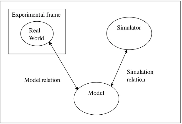
The conceptual framework of DEVS is shown in Figure 3.1. Basically, the modeling
and simulation concerns three basic objects including experimental frame, model, and
simulator. From the figure, we know that the real world is the fundamental data source,
and the experimental frame specifies the constraints to define the system under
experiment and study. The model is a series of instructions and structures to represent the
real system, and the simulator can be seen as a device to execute the model. Modeling
relation connects the real world and the model, which specifies how well the model
represents the real world. Simulation relation, linking the model and the simulator,
denotes how the simulator executes the instructions and structures.
Experimental frame
Real World
Simulator
Model
[image:31.612.153.463.430.642.2]Simulation relation Model relation
3.1.2 DEVS formalism
Formalism represents the structure of a model in mathematics. In DEVS formalism,
mathematical models are used to define the events occurrence at different times. There
are two kinds of models in DEVS formalism, the atomic model and the coupled model.
An atomic model is a structure as shown in equation (3.1).
M X,S,Y,δint,δext,δcon,λ,ta, (3.1)
where X is the set of input values; S represents a set of states; Y defines the set of output
values; int: S S is the internal transition function; ext: Q Xb S is the external
transition function, where Q {(s, e)| s S, 0 eta(s)} is the set of all the states, e is
the elapsed time since the last transition, Xb denotes the collection of bags over X; con: S Xb S is the confluent transition function; : S Yb is the output function; ta: S
R0+ is the time advance function. A coupled model is composed of atomic models
defined as shown in equation (3.2).
NX,Y,D,{Mj},Cext,Cint,Cout,Select , (3.2)
where X is the set of input events; Y is the set of output events; D is the name set of
subcomponents; {Mj} is the set of subcomponents, where for each i D, Mi is either an
atomic model or a coupled model; Cext D i i
X X
is the set of external input couplings;
Cint D i i D i i X Y
is the set of input couplings; Cout
φ
Y Y
D
i i is the external output
couplings function; Select: 2D D is the tie-breaking function which defines how to
select the event from the set of simultaneous events. The system can be modeled using
3.1.3 Applications of DEVS
Since it was proposed, DEVS has been used to model both continuous and discrete
systems, such as knowledge-based control of industry products, autonomous agents
systems, construction systems, supply-chain systems, systems biology, and
hardware/software systems. In Le Goc and Frydman (2003), SACHEM, a real time
intelligent diagnoses system based on DEVS paradigm was proposed. It provided a
framework for knowledge-based control of steel production, and it was a successful case
to use DEVS formalism in industry to save money up to millions of euros annually. In
El-Osery et al. (2002), a virtual laboratory for multi-physics agents was built based on four
components, computer networks, CORBA, DEVS, and soft computing methods (e.g.,
reasoning logic) from bottom to top. DEVS is also used in construction simulations, for
example, Palaniappan et al. (2006) used DEVS framework to analyze the workflow
between various trade contractors in production home building. To gain efficiency, it is
necessary to study the dynamic changes in supply-chain systems. Therefore, DEVS is
adopted in some supply-chain systems to analyze the complex interactions. Huang et al.
(2009) presented an application of DEVS formalism in semiconductor manufacturing
supply-chain systems, exploring the complex relationships between control policies and
manufacturing processes. System biology focuses on analyzing the behavior and
interrelationships between entities of entire functional biological systems. Towards this
goal, Uhrmacher and Priami (2005) adopted both DEVS and -calculus approaches to
analyze multiple relationships to study the biological systems. In addition,
hardware-in-the-loop applications can benefit from DEVS framework. In Glinsky and Wainer (2004),
hardware, facilitate the testing purpose in a risky environment, and support component
reuse in hybrid hardware/software systems using DEVS formalism.
Due to its wide use in many applications, DEVS has become a simulation tool in a
variety of implementations. DEVSJAVA (Zeigler and Sarjoughian 2002) is an object
oriented M&S environment based on Java language and DEVS formalism. Another
implementation of DEVS is DEVSC++ (Zeigler et al. 1996). These provide conveniences
for people to model the applications in their fields.
3.2 Wildfire spread model using DEVS — DEVS-FIRE
Based on DEVS formalism, the Rothermel’s model is chosen in the wildfire spread
simulation because it has been extensively validated and proven to be stable and robust
(Rey 2004). The following subsections will explain some important aspects of
DEVS-FIRE.
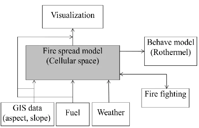
3.2.1 System architecture of DEVS-FIRE
The DEVS-FIRE model is an integrated environment for surface wildfire spread and
containment, built on Discrete Event System Specification (DEVS) formalism (Zeigler et
al. 2000). The overall structure of DEVS-FIRE is shown in Figure 3.2. From the figure
we know that the fire spread model is the core of DEVS-FIRE, which is modeled as a
cellar space containing neighbored cells with initialized fuels and the GIS data. When a cell is ignited, Rothermel’s model (the Behave model) is used to compute the speed and
direction of fire spread. Built on the fire spread model, DEVS-FIRE also supports fire
containment simulation by connecting to the fire fighting model. More details about the
fire containment simulation can be found in (Ntaimo et al. 2008). The visualization
3.2.2 Cellular space model of DEVS-FIRE
In DEVS-FIRE, the forest is modeled as a two-dimensional cell space containing a
series of rectangular cells whose dimensions depend on the resolution of the GIS fuel and
the terrain data. The fuel, terrain, and weather conditions within individual forest cells are
assumed to be constants (in the current model, the weather is assumed to be uniform for
the entire area). Each cell can be seen as a DEVS atomic model during the duration of
simulation and locally calculates the rate of speed and the direction based on the
parameters of fuel model, slope, aspect, and the weather data. Each cell has eight
neighboring cells according to the Moore neighborhood. The entire cell space is a
coupled model by connecting input ports and output ports between neighboring cells,
through which a cell can send messages to ignite its neighbor cells. The behaviors of
burning cells depend on both external inputs from their neighbors and the dynamic Figure 3.2 Structure of DEVS-FIRE
[image:35.612.143.472.91.303.2]change of the weather data, which is globally passed on to all the cells in the cell space
model.
Initially all the cells are set to the state of unburned (passive). If a cell receives an
ignition message and its fireline intensity is larger than the burning threshold, its state
will be changed to burning. After the burn delay time has elapsed, the burning cell
changes to the burned state. This time delay depends on the size of the cell and the fire spread speed, which is computed using Rothermel’s fire Behave model. As a result, fire
spread is modeled as a propagation process that burning cells ignite their unburned
neighboring cells. The state transitions of forest cells are displayed in Figure 3.3. In the
figure, the state transitions for fire spread are explained. For the fire suppress part of
DEVS-FIRE, related states (others) are needed, and not included here. Rothermel’s fire
behavior model is a semi-empirical mathematical model. In a small area and short-time periods, the fuel is taken to be homogeneous. The outputs of Rothermel’s model include
the rate of spread, the direction of maximum spread, flame length, and fire intensity that
measures the rate of heat released by a fire. In DEVS-FIRE, the rate (and direction) of spread from Rothermel’s model is then decomposed into eight directions including North,
NorthEast, East, SouthEast, South, SouthWest, West, and NorthWest from the ignition
point according to an elliptical shape as illustrated in Figure 3.4. The shape of this ellipse
is computed by the midflame wind speed and the fire spread rate (see (Finney 1998)).
Note that in Figure 3.4, we assume the maximum rate of spread is in the South direction.
The fire spread model of DEVS-FIRE has been partially validated by comparing with
NE N
NW
W E
SE
S SW
Ignition point
[image:37.612.114.503.79.365.2]Maximum rate of speed
Figure 3.4 Decomposition schema of DEVS-FIRE
Burned Burning
Unburned
Others
Others
Attack rules Fireline intensity >
threshold and ignition
Burned delay elapsed Attack rules
[image:37.612.179.452.439.684.2]3.2.3 Specification of DEVS-FIRE
As described above, the fire spread model of DEVS-FIRE is a cellular space model.
Each cell is modeled as an atomic model, and is coupled with its eight neighbors except
the boundary cells to form a cell space. Therefore, the cell space is as a DEVS coupled
model consisting of all the cells. In the DEVS formalism, a forest cell FC can be defined
according to (Zeigler et al. 2000) as shown in equation (3.3).
FC X,Y,S,δext,δint,δcon,λ,ta,xID,yID, (3.3)
where X is a set of inputs from its neighbors or weather inputs such as wind speed and
direction used in calculation; Y defines the set of outputs, which contains the data fed into
its neighbors for computation; S represents the cell’s states, for example, unburned,
burning, and burned during the fire spread; ext, int, and con represent the external
function, the internal function, and the confluent function respectively. These functions
are used to specify the state transitions for the forest cell; refers to the output function,
defining the outputs based on the cell’s states; ta specifies the time advance; and xID, yID
are the coordinates of the cell.
After coupling all the forest cells, we form a forest cell space coupled model, which
can be specified as shown in equation (3.4) according to the DEVS formalism.
FCS X,Y,D,B,N,Cext,Cint,Cout,r , (3.4)
where X and Y are the set of input events and output events respectively; D defines the set
of all the indexes in the cell space; B refers to all the boundary cells; N specifies the
neighborhood of the cell space, which is the Moore neighborhood, 8 neighbors for each
cell in DEVS-FIRE; Cext, Cint, and Ccon are internal couplings, external input couplings,
which is the size of each cell. The used DEVS-FIRE model was implemented in the
DEVSJAVA environment (Zeigler and Sarjoughian 2002).
3.2.4 Interface of DEVS-FIRE
From the structure of DEVS-FIRE, we know that the inputs should be specified
including the slope, the aspect, the fuel model, the weather condition, ignition points, and
running time. In DEVS-FIRE, we use a cellular space to represent the fire field.
Therefore, we also need to define the sizes of cellular space and each cell. Then, to define
the slope, aspect, and the fuel model of this cell space, three text files are needed. In each
file, a matrix whose dimensions are the number of cells horizontally and vertically is used
to specify slope, aspect, and fuel model values of all forest cells in the cell space. The
weather conditions are also defined by a text file, in which the wind speeds, wind
directions, and the moistures at different times are contained. During the two adjacent
time steps, the weather conditions are treated as the same. The ignition points are given
by the coordinates of cells that are initially burned. The running time means the time
period of the DEVS-FIRE’s execution.
The outputs of DEVS-FIRE include fireline intensities, burning perimeters, burning
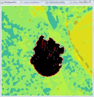
areas, etc. of the cells. The graphical output of the fire spread is a fire map, which represents all the cells’ states after the running time. In addition, the burning perimeters
and burning areas of can be captured at intervals. For example, assume we have a cell
space of 382 266 whose cell size is 30 30, and the aspect, the slope, and the fuel
model are defined using three text files, which are displayed in Figure 3.5. If the weather
conditions are that the wind speed is 5 miles/hour and 180 degrees (from South to North)
with the ignition point of the center in the cell space (191, 133). In the figure, the black
and red cells represent the burned and burning cells respectively, and all others are
unburned cells. Therefore, by the graphical interface, we can clearly figure out the
[image:40.612.166.466.182.494.2]situation of the fire growth.
CHAPTER 4 MEASUREMENT MODEL
The measurement model converts the output from the system model into the
measurement data, which is used to compare with the real time data. In this work, we
intend to estimate the evolving fire front, which represents the most important
information in a wildfire spread simulation. For the measurement data, we collect the real
time temperatures of distributed ground sensors in the fire field. Figure 4.1 shows how
the real time data is collected on-site using ground fire sensors. In the entire cell space, a
number of ground fire sensors are deployed.
GPS satellite
Sensor Data station
Each time step, fire sensors send messages including their positions and temperature data
to the data station, thus to provide real time data for fire scientists to analyze and use.
Based on the collected data in this context, the measurement model is defined as follows.
The measurement model maps the system state (the fire front) to the measurement
data (temperatures of deployed sensors). In DEVS-FIRE, the wildfire field is represented
by a discretized cellular space where the burning cells on the fire perimeter form the fire
front. Within this context, the measurement model includes two main aspects: the
deployment schema of ground temperature sensors, and the function of computing sensors’ temperature data from a fire front. The deployment schema defines how the
sensors are deployed in the wildfire field. Examples of deployment schema include
regular deployment, e.g., one sensor every 10 cells or every 20 cells, random deployment
where sensors are randomly distributed in the cell space, and fire-directed deployment
where more sensors are deployed around the active fire regions. These deployment
schemas (and the total number of sensors) result in different locations of the sensors. This
location information is used in computing the temperature data of the sensors.
4.1 Computation of temperatures
In (Kremens 2003; Mandel et al. 2008), time-temperature profile is studied and
assimilated. From these researches, we can know that the temperature will shapely
decrease with the increase of time and distance to the fire center as shown in Figure 4.2,
which can be denoted by the formula as shown in equation (4.1).
a x
x
ce T
T
T
2 2 0) (
σ , (4.1)
where T is the temperature of the sensor; Tc refers to the temperature rise above ambient
sensor, and x0 denotes the location of the closest burning cell on the fire front to the
sensor. Especially, Mandel et al. (2008) calibrates the relationship between the
temperature and the distance to the center and conclude the related empirical values,
which will be adopted in this measurement model.
To compute Tc for a burning cell, equation (4.2) is used (Van Wagner 1973; Van
Wagner 1975).
Tc 3.9FI /h
3 2
, (4.2)
where FI is the fire intensity of the burning cell (kW m-1) and h is the height above
ground (m). In the DEVS-FIRE simulation, the fire intensity of a burning cell is obtained from Rothermel’s Behave model. For ground temperature sensors, the height h would be
their installation heights.
0 100 200 300 400 500 600 700 800 900
35 50 65 80 95
T
em
pera
ture
(
T
c)
[image:43.612.177.439.207.475.2]Distance (m)
4.2 Example of the measurement model
To illustrate how the measurement model works to compute the temperatures of
ground fire sensors, we give an example as displayed in Figure 4.3. It shows a snapshot
of a fire spread simulation at some time point, when 8 cells are burning (display in red) in
the 9 9 cell space with each cell’s resolution being 15 meters. The temperature sensors
are regularly deployed in the cell space, i.e. one fire temperature sensor for every three
cells. In the figure, the cells that have deployed sensors are displayed in gray color. To
illustrate how the temperatures are calculated, we use the formula T 376ed2/2σ2 27
(let = 50) to specify the relationship between the distance from the sensor to the closest burning cell and the sensor’s temperature. Based on this formula, we can obtain the
temperatures of all the sensors, which are {149, 267, 267, 267, 386, 386, 267, 386, 371}
indexing from left to right, and top to bottom. Note that in this example, the closest
distances to the fire front for these sensors are {75, 45, 45, 45, 15, 15, 45, 15, 21}.
Burning cell
Cell with sensor
4.3 Sensor deployment schema
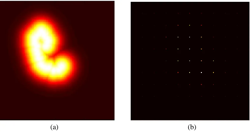
To illustrate how the different deployment schema can affect the temperature data
collected from sensors, Figure 4.4 shows the sensors’ temperature data for a given wildfire in three different deployment schemas, in which the sensor’s temperature varies
smoothly from black through shades of red, orange, and yellow, to white. In the figure,
Figure 4.4(a) is the real temperature map of a wildfire in a 200 × 200 cell space. This is
computed by assuming each cell has a temperature sensor deployed. In reality, much
smaller number of sensors will be used, and sensors will be deployed only to certain
locations in the wildfire field. Figure 4.4(b), Figure 4.4(c), and Figure 4.4(d) show the
temperature data for three different deployment schemas. In Figure 4.4(b), sensors are
regularly deployed with one sensor every 20 cells. Overall 100 sensors are deployment in
the cell space. Figure 4.4(c) and Figure 4.4(d) use the same number sensors. However, in
these two cases the sensors are randomly deployed. In the figures, for the two case of 100
sensors randomly deployed, we denoted them as Temperature map 1 and Temperature
map 2 respectively.
[image:45.612.98.509.494.716.2]
(c) (d)
[image:46.612.93.511.77.303.2]CHAPTER 5 DATA ASSIMILATION IN DEVS-FIRE SIMULATION
To present the data assimilation framework using SMC methods based on the
DEVS-FIRE model, we first formulate the data assimilation problem for applying SMC
methods. Then we present the procedure of SMC methods, including the sampling,
weight computation, and resampling stages of the procedure and their associated
algorithms, for assimilating data in DEVS-FIRE simulations.
5.1 Problem formulation
To improve the results of DEVS-FIRE wildfire spread simulations, the real time
data from real wildfires is assimilated into the simulation model. To apply SMC methods
for data assimilation, the system model of state evolution and the measurement model
that maps system state to measurement data need to be defined. Based on the
DEVS-FIRE simulation model, we formulate a non-linear state-space model as shown in
equation (5.1). . ) , ( , ) , ( 1 t t t t t t w t fire MM TM v t fire DF fire (5.1)
In equation (5.1), firet and firet+1 are the system state variables of fire spread at time step t
and time step t+1 respectively. In this work, we define the system state variable as the
evolving fire front, which is the most important information in a wildfire spread
simulation. Specifically, the fire front at time step t (firet) is composed of all the burning
cells along the fire perimeter at time step t. These cells ignite their unburned neighbors in
the wildfire spread simulation. They represent the initial condition for the simulation to
proceed to the next time step t+1. In our implementation, the fire front is specified by a
vector that includes the (x, y) IDs of all the cells on the fire front. TMt is the measurement