Influence of solar forcing, climate variability and modes of low frequency atmospheric variability on summer floods in Switzerland

www.hydrol-earth-syst-sci.net/19/3807/2015/ doi:10.5194/hess-19-3807-2015

© Author(s) 2015. CC Attribution 3.0 License.

Influence of solar forcing, climate variability and modes of

low-frequency atmospheric variability on summer floods in

Switzerland

J. C. Peña1, L. Schulte2, A. Badoux3, M. Barriendos4, and A. Barrera-Escoda1 1_{Meteorological Service of Catalonia, Barcelona, Spain}

2_{Department of Physical and Regional Geography and ICREA, University of Barcelona, Barcelona, Spain}

3_{Mountain Hydrology and Mass Movements Research unit, Swiss Federal Institute for Forest, Snow and Landscape Research} WSL, Birmensdorf, Switzerland

4_{Catalan Institute of Climate Sciences (IC3) and Department of Modern History, University of Barcelona, Barcelona, Spain}

Correspondence to: L. Schulte ([email protected])

Received: 2 December 2014 – Published in Hydrol. Earth Syst. Sci. Discuss.: 19 December 2014 Revised: 5 May 2015 – Accepted: 20 August 2015 – Published: 10 September 2015

Abstract. The higher frequency of severe flood events in Switzerland in recent decades has given fresh impetus to the study of flood patterns and their possible forcing mech-anisms, particularly in mountain environments. This paper presents a new index of summer flood damage that considers severe and catastrophic summer floods in Switzerland be-tween 1800 and 2009, and explores the influence of exter-nal forcings on flood frequencies. In addition, links between floods and low-frequency atmospheric variability patterns are examined. The flood damage index provides evidence that the 1817–1851, 1881–1927, 1977–1990 and 2005–present flood clusters occur mostly in phase with palaeoclimate prox-ies. The cross-spectral analysis documents that the period-icities detected in the coherency and phase spectra of 11 (Schwabe cycle) and 104 years (Gleissberg cycle) are related to a high frequency of flooding and solar activity minima, whereas the 22-year cyclicity detected (Hale cycle) is as-sociated with solar activity maxima and a decrease in flood frequency. The analysis of low-frequency atmospheric vari-ability modes shows that Switzerland lies close to the border of the principal summer mode. The Swiss river catchments situated on the centre and southern flank of the Alps are af-fected by atmospherically unstable areas defined by the pos-itive phase of the pattern, while those basins located in the northern slope of the Alps are predominantly associated with the negative phase of the pattern. Furthermore, a change in the low-frequency atmospheric variability pattern related to the major floods occurred over the period from 1800 to 2009;

the summer principal mode persists in the negative phase dur-ing the last cool pulses of the Little Ice Age (1817–1851 and 1881–1927 flood clusters), whereas the positive phases of the mode prevail during the warmer climate of the last 4 decades (flood clusters from 1977 to present).

1 Introduction

The response of floods to global changes is complex and can vary on a regional scale. Extreme flood event frequency can be highly sensitive to modest environmental and cli-mate changes (Knox, 2000), so much so, in fact, that these changes might not be recorded by mean hydrological values but rather by a changing pattern in the magnitude and fre-quency of extreme events (Benito et al., 2005). Moreover, these changes often occur during transitional stages of cli-matic pulses (Knox, 2000; Glaser and Stangl, 2004; Schulte et al., 2009a) and may respond to complex exogenic, endo-genic and autoendo-genic climate forcing mechanisms (Versteegh, 2005). Yet, the debate concerning the factors and trends that might influence flood dynamics, such as the rise in tempera-ture, river management and other human activities, remains a controversial one (Brázdil et al., 2006).

of glacial ice and snow cover, the outburst flood of lakes dammed by landslides as well as by other phenomena. The Alps are highly sensitive to changes in atmospheric circula-tion and environmental perturbacircula-tions that influence the hy-drological regime and flooding patterns reconstructed from instrumental data and documentary sources (Hächler-Tanner, 1991; Röthlisberger, 1991; Gees, 1997; Pfister, 1999; Luter-bacher et al., 2004; Weingartner and Reist, 2004; ALP-IMP, 2006; Burger, 2008; Schmocker-Fackel and Naef, 2010a, b; Wetter et al., 2011) and, regarding longer time series, from natural proxies such as lacustrine records, glaciers, den-drochronology and isotopic studies of speleothems (Tinner et al., 2003; Casty et al., 2005; Holzhauser et al., 2005; Boch and Spötl, 2008; Wilhelm et al., 2012). Referring to the last three millennia, solar activity may be an important driver of alpine floods as indicated by the periodicities (Gleissberg solar cycles) of geochemical and pollen proxies of alluvial plain sediments in the Swiss Alps (Schulte et al., 2008, 2015) and by their correlation with climate proxies.

During the last 500 years, periods of large floods have been reported by detailed documentary inventories and in-strumental series compiled by Röthlisberger (1991), Hächler-Tanner (1991), Gees (1997), Pfister (1999), Lehmann and Naef (2003), Vischer (2003), Burger (2008) and Hilker et al. (2009). According to the annual number of floods used by Schmocker-Fackel and Naef (2010a, b) as a parameter for the evaluation of the climate and hydric variability of catchments in Switzerland, increased flooding occurred dur-ing four main periods: 1560–1590, 1740–1790, 1820–1940 and 1970–2007. Since the second half of the 19th century, river correction and embankment may have influenced the frequency of flooding in the Swiss catchments. Other stud-ies discuss the possible links between hydrological extreme events and low-frequency atmospheric variability patterns (Pfister, 1999; Jacobeit et al., 2006; Knox, 2000; Glaser and Stangl, 2004; Mudelsee et al., 2004; Schmocker-Fackel and Naef, 2010b; Wilhelm et al., 2012), such as the North At-lantic Oscillation. However, in the Swiss Alps, floods show a strong seasonal distribution recording highest frequencies during the summer months. Summer climate in the North Atlantic-European sector possesses a principal pattern of year-to-year variability which is defined as the main empir-ical orthogonal function (EOF1) of the standardized anoma-lies of the European mean sea level pressure (EMSLP) dur-ing July and August. The location of the action centres shows strong positive anomalies (high pressure centre) between the Scandinavia Peninsula and Great Britain, while the Mediter-ranean region is dominated by light negative anomalies (low pressure centre). The EOF1 exerts a strong influence on rain-fall, temperature and cloud cover through changes in the po-sition of storm tracks in the North Atlantic region (Folland et al., 2009), but also in many areas of southern Europe (Bladé et al., 2011).

Our study aims to investigate the possible links between flood frequency in Switzerland and solar forcing, volcanic

eruptions, climate variability and the North Atlantic dynam-ics over the last two centuries. A study of summer flood fre-quencies in Switzerland has been conducted for the period 1800–2009, based on the calculation of a flood damage index (henceforth INU) from existing flood inventories for Switzer-land, summarizing both the severity of these events and their spatial extent. Special attention will be focused also on the possible different evolution between flood dynamics at the northern and southern slopes of the Alps during the last two centuries. The influence of solar forcing on flood frequen-cies is investigated, applying a cross-spectral analysis to the sunspot record and INU to determine the common period-icities, and we used temperature reconstructions, volcanic eruptions, beryllium-10 records (solar activity) and oxygen isotope data (Greenland climate proxies) for finding links. Finally, the analysis of the possible links between floods and North Atlantic dynamics is focused on the low-frequency at-mospheric variability pattern (EOF1).

2 Data and methods 2.1 Historical flood data

Historical descriptions of flood events are reported in the Alps by local monographies, chronicles, Council minutes, manuscript sources and specialized literature, and from the 18th century onwards, by press and expert reports (Pfister, 1999). Instrumental discharge measurements of gauge sta-tions started in Switzerland mostly at the beginning of the 20th century.

To explain the variability and frequency of floods in Switzerland between 1800 and 2009, an integrated flood damage index (INU) was calculated from two data sources: a flood database, provided by Gees (1997) for the period 1800– 1994, which were developed from the historical records com-piled by Röthlisberger (1991), Pfister and Hächler (1991) and further historical investigation; and selected flood damage data extracted from the Swiss flood and landslide damage database of the Swiss Federal Institute for Forest, Snow and Landscape Research, WSL for the period 1972–2009 (Hilker et al., 2009). The contemporary flood series of the WSL, gen-erated from damage events reported by the local, regional and national press and websites (police, fire department, etc.), were transformed according to the database structure of Gees (1997) to extend the flood index.

Based on this information, we built a database with a ma-trix structure, A (M×N), where M rows state the event date and each of theN columns reports the flood informa-tion for each of the Swiss cantons. The cells from which the matrix is comprised then either bear a code or are left empty, depending on the incidence of a flood event on the given date and in the specific canton. The code reports the flood category, based on the damage in Switzerland quanti-fied in millions of Swiss francs (CHF) taking inflation into account (Gees, 1997; Hilker et al., 2009). A flood is con-sidered a low-damage event (L) if the damage is calculated at less than CHF 0.2 million; a medium-damage event (M) if the damage is between 0.2 and 2 million; a severe-damage event (S) if the damage is between 2 and 20 million; a very severe-damage event (VS) if the damage is between 20 and 100 million; and a catastrophic-damage event (C) when the damage caused by the flood event exceeds CHF 100 million. Difficulties with regard to the homogeneity of historical flood time series are expected due to the lower precision and possible data gaps of flood records from earlier periods. However, Gees (1997) showed that this heterogeneity mostly affects the small and medium category floods, whereas the very severe and catastrophic events have not shown this ef-fect since the increased sensibility of the population caused by the increased floods during the first half of the 19th cen-tury, the application of the Swiss Federal Law on River Cor-rection since 1854 and the improved information transmis-sion by the press. Moreover, flood mitigation management such as levee construction, retention reservoirs and river de-tour into large lakes may have had an influence on flood frequency since the 18th century and improved since 1900 (Wetter et al., 2011). Other factors such as ground sealing, canalizing riverbeds and exposure of public infrastructure increased runoff, discharge and economic losses during the 20th century. It is difficult to estimate how these opposite effects partially compensate for each other (Pfister, 1999). It is important to state that the improved river regulation in Switzerland, conducted from 1850 onwards, may mitigate the damage caused by low, medium and major floods, but cannot prevent completely the total impact of category VS and C floods as occurred for example during the 1987 and 2005 events. From our research on flood dynamics and evo-lution of delta morphology of the Lütschine and Hasli Aare rivers starting from 1480 (Schulte et al., 2015), we observe the same trend: the frequency of very severe and catastrophic floods does not show a substantial change, whereas small and medium floods are recorded with improved precision after 1800. Therefore, we use only the very severe (VS) and catas-trophic (C) flood events to generate the flood damage index (INU). To validate the historical flood data, in order to build the INU index, all events of category VS and C were checked if they were cited by different sources and if damage occurred simultaneously in different sites. From 91 events, only the event of 4 August 1868 was excluded. The flood database of the WSL (1972–2009) is considered to be complete.

2.2 Instrumental and proxy data

Solar forcing is considered an external driver of climate dy-namics (Stuiver et al., 1997; Versteegh, 2005) and may in-fluence flood frequency (Benito et al., 2003; Schulte et al., 2008, 2015). Average annual sunspot numbers (SN) for the period 1700-2011 were downloaded from the online cat-alogue of the sunspot index provided by the SIDC team (World Data Center for the Sunspot Index, Royal Obser-vatory of Belgium, Monthly Report on the International Sunspot Number). To complete this analysis, we used a solar proxy, the annual mean values of the beryllium-10 records (10Be) measured in the ice core from the NGRIP site in Greenland (Berggren et al., 2009). Deposition of atmospheric 10_{Be into polar ice sheets is a natural archive with annual} res-olution about past solar activity and constitutes a proxy for understanding possible connections between solar variability and past climate change (Beer et al., 2000; Berggren et al., 2009).

Volcanic eruptions are investigated by mean volcanic phate deposition and converted to stratospheric volcanic sul-phate injection (in Tg units) for the Northern Hemisphere over the past 200 years (1800–2000). These measures have been extracted from 32 ice core records that cover a major part of the Greenland ice sheet (Gao et al., 2008).

Climate variability is analysed from a climate proxy, the annual mean values of the oxygen isotope recordδ18O for the period 1800–1987 from the Greenland ice core GISP 2 (Stuiver and Grootes, 2000). This core provides climate in-formation based on conversion of isotope values to mean an-nual temperature in Greenland. Furthermore, we determined the average annual temperature for Switzerland from 1800 to 2006 based on data obtained from the EC project: multi-centennial climate variability in the Alps (ALP-IMP, 2006). This data set is based on instrumental data, model simula-tions and proxy data, with the purpose of creating a spatial grid of several climate variables. The average temperature was obtained by calculating the arithmetic mean of the grid points corresponding to Swiss territory.

A complete reference list of web links to the different data sets used in the analysis is given at the end of the manuscript.

3 Methods

Given the hydro-climatic differences according to the singu-lar orographic configuration of Switzerland, the trigger pro-cesses of floods, especially rainfall generation propro-cesses, are different between the northern and southern flank of the Alps (Schmocker-Fackel and Naef, 2010). Although there are sev-eral Swiss climatologic and hydrologic regionalization stud-ies (e.g. Kirchhofer, 2000), we conducted a regionalization of the Swiss territory based on a multivariate data analysis. The input data were performed by the matrix of INU (see Sect. 2.1.1). To identify the principal hydro-climatic regions, we applied principal component analysis (PCA) to the flood matrix in S mode using the correlation matrix. The critical as-sumptions underlying PCA are more conceptual than statisti-cal. Only normality is necessary if a statistical test is applied to the significance of the factors. The data matrix should en-sure that sufficient correlations exist to justify the applica-tion of factor analysis (Hair et al., 1998). Two tests were used to evaluate the model: the Kaiser–Meyer–Olkin mea-sure of sampling adequacy (KMO) and Bartlett’s sphericity test. The KMO statistic varies between 0 and 1. A value close to 1 indicates that patterns of correlations are compact and therefore PCA should yield distinct and reliable factors. Ac-cording to Kaiser (1974) the recommended acceptable values should be greater than 0.5. If the KMO value is less than 0.5 we can evaluate the anti-image correlation matrix to delete redundant variables (that is to say, those variables that have values less than 0.5 in the principal diagonal) to improve the results of PCA. Bartlett’s sphericity test checks the presence of correlations among the variables. It tests the null hypoth-esis that the correlation matrix is an identity matrix, i.e. all diagonal elements are 1 and all off-diagonal elements are 0, implying that all of the variables are uncorrelated. If the sig-nificance value (sig. value) for this test is less than our alpha level (α), we reject the null hypothesis. Finally, we used the scree test to extract the most relevant components and the equamax normalized rotation for a straightforward interpre-tation of the model output. This rointerpre-tation is a compromise be-tween varimax and quartimax. Specifically, it maximizes the sum of variances of the squared raw factor loadings across factors and the same process across variables. This is equiva-lent to simultaneously maximizing the variances in the rows and columns of the matrix of the squared raw factor loadings. INU is calculated separately for each of the regions de-termined from the PCA by evaluating the different spatial and temporal patterns that account for the variability in the frequency of floods. The INU is estimated taking a risk (R) approach, whereby the concept of risk (R) is considered to be the product of hazard (P) and vulnerability (V):

R=P·V . (1)

The variableP is estimated from the damage and economic losses caused by floods. The categories of damage are as de-fined in Sect. 2.1.1. To each category an arbitrary magnitude is attributed: floods classified as VS are given a value of 50, while C floods are assigned a value of 100. Thus, each flood event is defined by aP value that indicates the intensity of the phenomenon. The estimation ofV, defined as the spa-tial distribution of the phenomenon, is based on the number of cantons affected by a flood episode. Finally, by applying Eq. (1) we obtain an R value for each flood event.

RK= m X

i=1

Pi∗Vi (2)

Kis the flood number (ordinal 1 toN whereN is the total number of floods),mis the number of the cantons concerned in the flood numberK,Piis the hazard of the flood numberk and the cantoniandVi is the vulnerability of the flood num-berK. In our caseVi=1 always. The INU is calculated from the integration of all theRvalues on an annual resolution:

INUyear= j X

i=1 n X

K=1

RK. (3)

INUyearis the INU value for a given year,j is the number of the months (1 to 12) andnis the number of events in a given monthj. Finally, each INUyearis standardized, based on the mean and standard deviation; both parameters are calculated for the period 1800–2009.

A further methodology is concerned with the definition of low-frequency atmospheric variability modes. Several au-thors use the main EOF calculated from principal component analysis (PCA) in S mode applied to the grid of EMSLP us-ing the covariance matrix (Hurrell et al., 2003; Folland et al., 2009; Bladé et al., 2011) and the scree test (Cattell, 1966) to extract the most relevant components without applying any kind of rotation. The analysis was conducted for the domain from 30 to 70◦N and from 30◦W to 30◦E for the period 1800–2009. To cover the entire period, we used the recon-struction of sea level pressure fields, weighted by the square root of the latitude over the eastern North Atlantic and Eu-rope, generated by Luterbacher et al. (2002) and the 20CRP (Compo et al., 2011).

4 Results

4.1 Regionalization of Switzerland and INU as a flood damage index

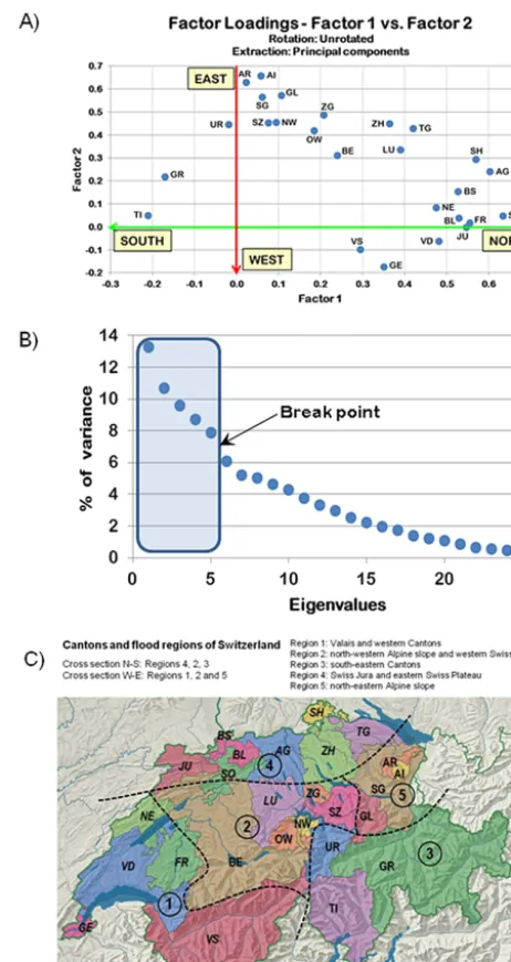
A total of 90 category VS and C floods were recorded in Switzerland in the period 1800–2009. The regionalization of Switzerland is based on the application of a PCA to the flood matrix. The KMO measure of sampling adequacy is 0.82, which would be labelled as very good. Since this measure meets the minimum criteria to evaluate the correlation pat-terns of the data set, we do not have a problem that requires us to examine the anti-image correlation matrix to delete the redundant variables of the analysis. The result of Bartlett’s sphericity test shows that sig. value=0.000 <α=0.05 (chi-square=2128.42, degrees of freedom=325). The sig. value for this analysis leads us to reject the null hypothesis and con-clude that there is no evidence that the correlation matrix is an identity matrix and the data set is appropriate for the appli-cation of the PCA. The 2-D plot of the two principal compo-nents (not rotated; see Fig. 1a) accounts for 22 % of the total variance. When the factors are inverted and rotated by 90◦, they display the geographic location of the cantons approx-imately. This two principal components can be interpreted as the two principal moisture sources that affect Switzer-land. Factor 1 is related to a disposition north/south of the cantons, indicating a lower/greater influence of the Mediter-ranean Sea. The second factor is explained by the west/east cross section, suggesting the higher/lower influence of the Atlantic moisture source.

We used the scree test to extract the most relevant compo-nents (see Fig. 1b) and we performed an equamax rotation in order to achieve the final regionalization of Switzerland con-sidering the two cross sections. The analysis revealed five principal components accounting for 45 % of the total vari-ance. Each region is defined by a component (see Fig. 1c): the region 1 is composed of the Valais and the western can-tons, region 2 is defined by the western part of the northern slope of the Alps and the western Swiss Plateau, region 3

Figure 1. (a) Factor loadings of factor 1 versus factor 2 after the ap-plication of the PCA to the flood matrix without rotation. (b) Scree test and number of components selected. (c) Regionalization of Switzerland according to the PCA, applying the equamax rotation. The dotted lines show the limits of the regions (DEM from Atlas of Switzerland, 2004; map modified).

distin-Figure 2. (a) Monthly distribution of major floods in Switzerland for the period 1800–2009 for very severe (VS) and catastrophic (c) flood categories. (b) Seasonal distribution of VS and C floods. DJF: December-January-February; MAM: March-April-May; JJA: June-July-August; SON: September-October-November.

guishes between the flows from the west-northwest and those from the north.

Figure 2 shows the monthly and seasonal distribution of VS and C events for the period 1800–2009. The monthly (Fig. 2a) and seasonal (Fig 2b) flood cycles are heavily pronounced: 65 % of these events are concentrated in the summer season (June, July and August), rising to 82 % if September is included (extended summer). Furthermore, the monthly distribution presents a peak in August with 37 % of all events. It should also be noted that during the months of March, April and December, no major floods were recorded. Recall, however, that the flood damage index only considers the events recorded during the high summer months (July and August). We proceed in this way for two main reasons: first, this is the time window considered by the EOF1, which is the principal pattern for explaining rainfall patterns in terms of large-scale atmospheric phenomena; and, second, most of the catastrophic floods (C; 60 %) reported during the time span of this study occurred during this 2-month period.

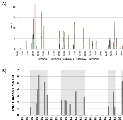
Figure 3a shows the annual flood damage index accord-ing to the contribution of each region. The INU captures the high temporal variability of floods showing the alternation of

high-frequency periods of major flood events and periods of very low frequency or flood gaps. The advantage afforded by the INU is that we are able to process the time series sta-tistically. Figure 3b shows the total annual INU values of the Switzerland and indicates periods with high frequency of flooding (grey shaded). Each column summarizes the infor-mation shown in Fig. 3a by using the following expression:

INUyear= N X

i=1 INUi,

! 1

N, (4)

where for a determined year,iis the region number, INUi is the INUyearfor the regioniandN=5 (total number of re-gions). Finally, the new data set is normalized by the mean and the standard deviation of the period 1800–2009. The ma-jor flood periods can be identified with respect to INU values that exceed the mean plus 1.5 times the standard deviation. The first period marked by a high frequency of major floods (Fig. 3b) extends from 1817 to 1851; the second period from 1881 to 1927, although some flooding did continue to occur, albeit less frequently, up to 1951 (Fig. 3a); the last two pe-riods were recorded from 1977 to 1990 and 2005 to present. Since that date, the 2005 flood event has caused the most severe damage (CHF 3.1 billion) followed by the 1987 flood (CHF 1.77 billion).

4.2 Spectral analysis of large floods

Figure 3. (a) Regional flood damage index INU for the period 1800–2009. (b) Values of INU that exceed 1.5 times the standard deviation. The periods with a high frequency of flooding are shaded grey.

4.3 Cross-spectral analysis between sunspot numbers and large floods

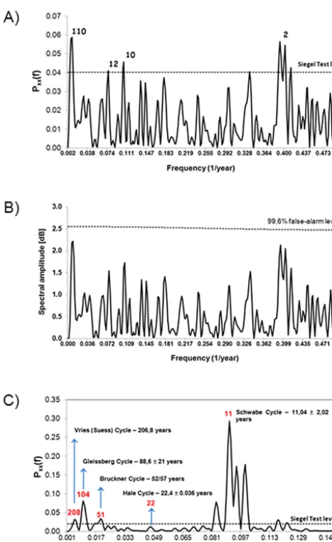
To compare the periodicities identified in the INU with cycles of solar activity, a harmonic analysis of the annual average sunspot number for the period 1700–2011 was conducted. The results show the main solar cycles on decadal and cen-tennial scales (Fig. 4c) and are consistent with the results of solar periodicities reported by Rogers et al. (2006). The INU shows common periodicities with solar cycles at 0.010 and 0.090, corresponding to 104 and 11 years, respectively.

To consider the significance of the common spectral peaks of INU and the sunspot record, a cross-spectral analysis was undertaken to obtain the coherency and phase spectra (Fig. 5). Since maximum values in the INU are expected to correlate with minimum solar activity values, as pointed out in a number of studies (e.g. Pfister, 1999; Magny et al.,

associ-Figure 4. (a) Harmonic analysis for the summer flood damage index INU. The dotted line represents critical level for the Siegel test and significant frequencies are shown in years. (b) Red noise AR1 spec-tra of INU. The dotted line shows false-alarm level. (c) Harmonic analysis for the average annual number of sunspots. The dotted hor-izontal lines represent critical levels for the Siegel test. Significant frequencies are shown in years. The principal solar cycles are high-lighted.

ated with maximum solar activity and a decrease in the flood frequency (positive angles in the phase-spectrum).

4.4 Comparison between modes of low-frequency atmospheric variability and large floods

The INU index provides an excellent tool to explore the space-time dependence between major floods in Switzerland and low-frequency atmospheric variability patterns. Dur-ing the high summer, the climate variability in the North Atlantic-European sector is synthesized by a major annual variability pattern identified as the EOF1. This pattern was detected by the first covariance eigenvector of EMSLP

com-Figure 5. Cross-spectral analysis between the index of summer flood damage INU and annual number of sunspots: (a) Coherency spectrum. Dashed line indicates false-alarm level for α=0.1. (b) Phase spectrum. The sign of the INU data was changed prior to cross-spectral analysis in order to prevent an artificial phase offset by±180◦. Negative angles indicate that the maximum frequency in the floods occurs during a solar activity minimum and vice versa.

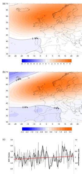
puted from a PCA in S mode, over the domain 30–70◦N and 30◦W–30◦E, with a monthly resolution for the two reanal-ysis grids used: 20CRP (Compo et al., 2011) for the period 1871–2009 (Fig. 6a), and the sea level pressure fields over the North Atlantic and Europe for the period 1659 to 1999 (Luterbacher et al., 2002; Fig. 6b). The low-frequency at-mospheric variability pattern obtained separately from both grids is quite similar, explaining roughly 40 % of the EMSLP variance. Both models are comparable to those presented by Folland et al. (2009, see Fig. 1, pp. 1085). Furthermore, the coefficients of the scores matrix report the temporal evolu-tion of the EOF1. The Pearson temporal correlaevolu-tion coeffi-cient between the scores of both time series has a value of 0.89. This level of association has allowed us to create the EOF1 index for the period from 1800 to 2009 (see Fig. 6c).

land. In addition, the positive phase of EOF1 detected in the 18th century coincides with the flood cluster between 1740 and 1790 reconstructed by Schmocker-Fackel and Naef (2010b). Only the high-frequency phase of major floods that was recorded during the first half of the 19th century (cf. Fig. 3b) is not reflected in the temporal evolution of the EOF1 data.

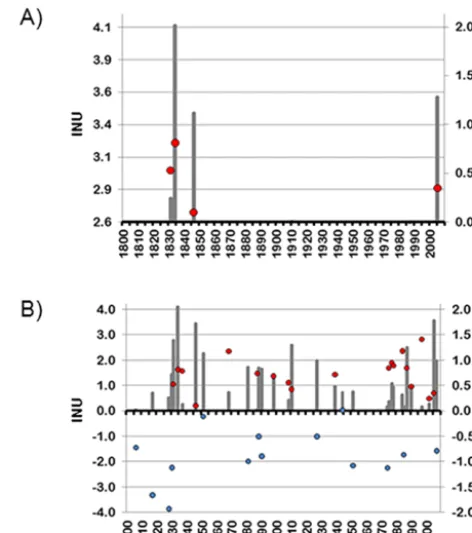
The increase in flood frequency occurs mostly in the pos-itive phases in the large-scale variability pattern for the high summer period. Flood events with INU > 5 SD (Fig. 7a) cor-relate with positive EOF1 values (Pearson’s temporal corre-lation coefficient is 0.45, significant at the 95 % confidence level). However, the study of the complete amplitude of the INU and EOF1 signals (Fig. 7b) indicates a second flood pat-tern during negative phases of EOF1. Table 1 shows the mean values of EOF1 for the years assigned to four categories of the INU whose thresholds were defined according to the standard deviation (from INU > 0 SD for at least one major flood to INU > 5 SD for highest flood impacts). The 33 sum-mers with very severe or catastrophic floods in Switzerland (INU > 0 SD) show a weak positive value of EOF1=0.04 (±0.90), which increases to 0.45 (±0.90) when considering only those summers that have recorded a flood with a large impact (INU > 5 SD). The number of years involved in INU > 0 with positive phase of EOF1 is also higher than the years associated with a negative phase (20 and 13, respectively), noting that the 4 years involved in the major floods all have a positive value of EOF1. However, with regard to a reliable explanation of the triggering processes for floods in Switzer-land which are based on large-scale atmospheric patterns, we also observe a significant number of years in the negative EOF1 phase. In addition, this is shown by the second per-centile (see Table 1) indicating negative values of EOF1 up to INU > 2.5 SD. In Sects. 5.1 and 5.4 we focus on the is-sue of whether the observed differences in the behaviour of the positive and negative EOF1 phases are linked to the two spatial patterns associated with the hydro-climatic regional-ization (see Sect. 5.1 and Fig. 8). Moreover, we briefly anal-yse whether there have been changes in low-frequency at-mospheric variability patterns associated with major floods during the last 200 years.

5 Discussion

5.1 Hydro-climatic regionalization and flood periods in Switzerland

The hydro-climatic regionalization performed by the PCA shows two patterns of spatial variability related to the two principal moisture sources that affect Switzerland: Mediter-ranean and Atlantic humidity supplies. The first pattern is related to the north–south cross section while the second pat-tern is defined by the west–east cross section (see Fig. 1a). Taking into account these findings, the final classification

Figure 7. (a) Summer flood damage index INU (bars) versus posi-tive phase of EOF1 (red dots) for values of INU 5 times greater than the standard deviation (INU > 5 SD). (b) As in (a) but for the com-plete signal of the INU. Blue dots represents negative EOF phase.

Figure 8. Cumulative number of floods (in %) versus time, for each region: the cumulative frequencies are obtained by adding the abso-lute frequencies of all years up to the year referred to. Black line: Bisector of the quadrant where the distribution of the floods is per-fect.

Table 1. Principal statistical parameters of EOF1 for each of the categories of the flood damage index INU whose thresholds were defined according to the standard deviation (SD).

INU_i> 0 SD INU_i> 1.0 SD INU_i> 2.5 SD INU_i> 5.0 SD

Average 0.04 0.10 0.18 0.45

EOF1+(years) 20 11 6 4

EOF1 – (years) 13 7 3 0

N 33 18 9 4

Max 1.41 0.94 0.84 0.81

Min −1.93 −1.12 −0.79 0.10

P95 1.18 0.90 0.83 0.77

P2 −1.76 −1.08 −0.74 0.12

the Atlantic flux and on the other hand the moist Mediter-ranean air masses that flow across the Alps and encounter the cooler Atlantic air at the northern Alpine slope (Pfister, 1999).

The regional distribution is consistent with other classifi-cations of Switzerland (e.g. Kirchhofer, 2000) that have been widely used such as for weather forecast and warnings for heavy rain (Schmocker-Fackel, 2010a). A major drawback of our classification is that regions have been constructed from administrative units (cantons) that in some cases may include different physiographic units. For example region 2 includes the canton Berne which range from the northern Alps to the Swiss Plateau and the southern slopes of the Jura Massif. However, the classification avoids the overestimation of the small Swiss cantons.

The temporal evolution of the regional INU shown in Fig. 8 indicates two spatial flood patterns: during phase A from 1820 to 1910 flood numbers increased in the basins of the west and northern flank of the Alps (region 1, 4 and 5), whereas during phase B from 1970 to the present floods in-creased in the centre and south of the Alps (regions 2 and 3). This decadal variability might be linked to changes in pat-terns of extreme precipitation and large-scale atmospheric variability (Frei et al., 2000). Schmocker-Fackel and Naef (2010a) suggest that this changing atmospheric pattern is not well defined for Switzerland yet.

The total INU index, summarizing the temporal distribu-tion of the frequency of very severe and catastrophic floods in Switzerland, presents four major flood periods: the first extends from 1817 to 1851, the second from 1881 to 1927, the third encompasses 1977 to 1990 and the fourth was initi-ated in 2005 (Figs. 3b and 9). These periods largely coincide with those reported in other studies for Switzerland (Hächler-Tanner, 1991; Röthlisberger, 1991; Gees, 1997; Pfister, 1999; Schmocker-Fackel and Naef, 2010b) and, furthermore, with the periods identified in Spain, Italy and the Czech Re-public (Barriendos and Rodrigo, 2006; Camuffo and Enzi, 1996; Brázdil et al., 2006). Our study shows that periods of high-frequency flooding have a period around 90 years. This range is very similar to that observed in Germany: for

in-stance, Glaser and Stangl (2004) report flood clusters that range between 30 and 100 years during the last millennium, whereas in northern Switzerland these periods have a dura-tion of between 30 and 120 years (Schmocker-Fackel and Naef, 2010b). In our opinion, the INU provides a robust in-dex, which captures the variability in major flood frequency, although the distribution of the clusters is not homogeneous in time.

Pfister (1999) who reconstructed the floods of the Rhine, Rhone and Reuss rivers and of Lake Maggiore from docu-mentary sources and instrumental data for the past 500 years found that major flood clusters occurred during cold peri-ods of the Little Ice Age. The last flood pulse from 1827 to 1875 corresponds to the first period identified in our study (1817–1851). However, the Little Ice Age also included pe-riods with no flood activity in alpine basins and which co-incided with periods of decreased solar activity, such as the Maunder Minimum (Pfister, 1999). As for the flood analysis undertaken by Schmocker-Fackel and Naef (2010b) in Swiss catchments, the alternation of periods of high and low flood frequencies coincides with those reported in our study.

cor-rection subsidies in 1848. However, there is a consensus in the literature that the older the event (and, hence, the associ-ated damage) is, the less clear the definition of the thresholds between the loss categories is.

A second flood gap is recorded from 1944 to 1972 by the INU reflecting the absence of extreme weather conditions (predominance of negative EOF1; Fig. 6c) that might trig-ger major floods. Pfister (1999) argues that anthropogenic influence (land use, deforestation) in the major floods is not the dominant driving factor, but rather the long-term sum-mer precipitation minima between 1935 and 1975. Accord-ing to Gees (1997), river regulation and the buildAccord-ing of em-bankments and reservoirs substantially reduced the damage caused by smaller and medium floods after 1854, whereas the mitigation of the impact of very severe and catastrophic floods showed only limited success, particularly in the up-per alpine catchments. Nevertheless, the more intensive land use in former flood areas protected by river embankments contributed to increased losses (Gees, 1997). Moreover, it is important to bear in mind that the general increase in popu-lation, exposure values (due to the increase in the gross do-mestic product) and urban agglomeration (e.g. Zurich) have contributed to higher flood damage indices, particularly in recent decades. A decrease in the number of floods is also re-ported by Schmocker-Fackel and Naef (2010b) for northern Switzerland between 1940 and 1970, and Wetter et al. (2011) observe a period of very low-frequency flooding in the city of Basel (Rhine river) for the period 1877–1999 and in Lindau (Lake Constance) for the 1910–1999 time interval.

Finally, the increase in flood events since 1977 recorded by the INU seems to have resulted from both increasing vulnera-bility and from changes in climate signal. With regard to this first factor, Glaser et al. (2010) found that even though the number of extreme hydrological events decreased compared to the 19th century, estimations of overall losses are substan-tially higher. This is related to the increased vulnerability and exposure values in flood prone areas as a consequence of the expansion of urban areas. As for the influence of cli-mate variability on flooding in recent decades, Knox (2000) stated that the unusually high frequency of large floods which has been observed in many regions since the early 1950s oc-curred during a period of global temperature increase, and that the occurrence of extreme floods during the Holocene is often associated with rapid climate changes. In Switzer-land, the flood frequency in many basins has increased since the 1970s (Gees, 1997; Pfister, 1999). However, Schmocker-Fackel and Naef (2010a) consider that the flood frequencies observed during the past 4 decades do not exceed the range recorded during the last five centuries.

5.2 Possible control of solar variability

In recent decades, the sun–climate relation has been anal-ysed (Solanki and Fligge, 2000; Versteegh, 2005; Gray et al., 2005), with solar variability being proposed as a possible

driving force of flood events (Benito et al., 2003; Vaquero, 2004). Schulte et al. (2008, 2015) consider the impact of so-lar activity on the regional hydrological regime (e.g. Gleiss-berg cycle) to have been one of the main factors triggering the major floods in the Lütschine and Lombach catchments in Switzerland over the last 3200 years.

By undertaking spectral analyses of the INU and the sedi-mentary proxies of the northern slopes of the Alps (Schulte et al., 2015), we are able to identify common flood cycles with a variation ranging between 70 and 150 years. The periodici-ties of so-called “100-year events” (according to Glaser et al., 2010) could be explained by centennial-scale solar cycles, which have also been identified in other sedimentary records, including those in eastern France, Switzerland, Netherlands, the UK, Spain and California (see, for example, Magny et al., 2003; Versteegh, 2005). Cross-spectral analysis between the INU and sunspot numbers suggests that the common and significant periodicities detected in the coherency spectrum of 11 (Schwabe cycle) and 100 years (Gleissberg cycle) co-incide with the relation between a high flooding frequency and minimum solar activity (negative angles in the phase spectrum). This fact is supported by the findings of Wirth et al. (2013a) in the reconstruction of the summer floods in the southern European Alps. Furthermore, the 22-year cyclicity detected (Hale cycle) includes the link between solar activity maxima and decreased flood frequency (positive angles in the phase spectrum). This bi-decadal frequency of the INU “flood minima” is confirmed by climate proxies in the west-ern United States where droughts occurred with a 22-year periodicity from 1700 onwards (Cook and Stockton, 1997; Briffa, 2000).

5.3 Short-term external forcing on flooding

To evaluate possible links between flooding and short-term external forcing fluctuations, the volcanic eruptions, EOF1,

et al., 2000). However, other proxies such as the δ18O are influenced by the oceanic thermohaline circulation besides solar activity. However, it must be taken into account that the length of INU time series is relative short, covering 200 years, and linkages are based on only four flood periods and three flood gaps. Therefore, the relation between INU and the different climate proxies must be interpreted with cau-tion and simple associacau-tions must not explain causal mecha-nism. Furthermore, it should be stressed that the INU signal includes uncertainties due to the integration of natural and anthropogenic variables. These reasons have to be borne in mind before discussing the following results.

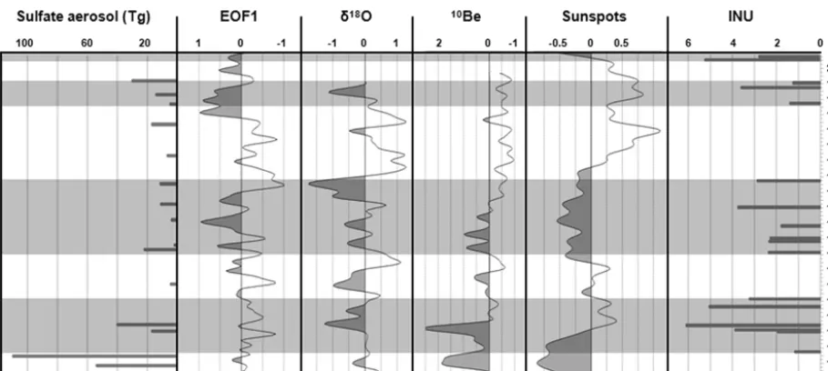
Three periods of low solar activity (low number of sunspots, positive anomalies of 10Be) have been recorded during the last 200 years (Fig. 9; cf. Solanki and Fligge, 2000; Berggren et al., 2009): the first period covers the years leading up to 1840, and corresponds to the final stages of the Dalton Minimum; the second period lasts from 1880 to 1910 (10Be) and 1935 (SN), corresponding to the solar min-imum of 1900; and a third period begins after 2005, reach-ing minimum values in 2009. Figure 9 provides evidence that the periods marked by a high flood frequency typically corre-spond to periods characterized by a predominance of positive 10_{Be anomalies and, therefore, associated with episodes of} low solar activity. This pattern was particularly strong dur-ing the solar minimum of 1900. The period of high flood frequency between 1817 and 1855 largely corresponds to a period characterized by positive 10Be anomalies, although the flood peaks occurred in the transition between a solar minimum and a solar maximum. During this period an ex-tra cooling occurred which was associated with the erup-tion of Tambora (1814) plus two eruperup-tions in the years 1831 and 1835 (Fig. 9). Considering both forcings (solar and vol-canic), the temperature anomaly for this period compared to the 1961–1990 mean was around −0.5◦C in the Northern Hemisphere (Gao et al., 2008) and −1.1◦C for the Swiss Alps (Büntgen et al., 2006). Finally, the maximum of the last flood cluster corresponds to a short period of low solar activ-ity after 2005.

Several authors (Pfister, 1999; Knox, 2000; Magny et al., 2003; Benito et al., 2003; Schulte et al., 2012; Ortega and Garzón, 2009) contend that the most significant variations in the frequency of flooding have occurred during cold mate phases, particularly during transitional stages of cli-matic pulses. This pattern has also been observed in Switzer-land during the last 500 years (Schmocker-Fackel and Naef, 2010b; Glur et al., 2013; Wirth et al., 2013a, b), although af-ter the 1970s the climate and flood pataf-tern changed. Theδ18O record GISP2 from Greenland (Stuiver and Grootes, 2000), influenced by North Atlantic dynamics, provides a proxy of the temperature variability in the middle and high latitudes of the Northern Hemisphere. The peak clusters of the flood damage index INU (Fig. 9) can be related to periods domi-nated by negativeδ18O anomalies (bearing in mind that the

axis is inverted), principally to the cooler pulses from 1830 to 1845, from 1880 to 1930 and during the 1980s.

To corroborate these results obtained from large-scale proxies, in Fig. 10 we plotted the normalized annual aver-age temperature of Switzerland for the period 1800–2009 vs. the INU. The first two flood clusters occurred during a period of negative temperature anomalies between 1825 and 1935. In addition, these two flood clusters are related to pulses of marked temperature decreases separated by a flood gap which corresponds to a period of temperature recovery (slightly negative temperature anomalies >−0.2◦C) and so-lar activity (Fig. 9). The flood peak of summer 1987 occurs in a period in which temperature anomalies in Switzerland were slightly positive, butδ18O was negative in Greenland, indicative as such of the influence of North Atlantic dynam-ics. The 2005 and 2007 floods occurred in a clearly warm phase in Switzerland, corresponding to a contemporary max-imum. However, the climatic interpretation of these events should be undertaken with caution because the final temper-ature data once again present a slight fall and sunspot num-bers clearly decrease. Yet, these data represent the end of the time series. As for the pattern of flood gaps, Fig. 10 provides clear evidence: gaps of floods (1852–1880; 1928–1976) are related to positive temperature trends. Moreover, the contem-porary flood cluster is divided by the positive trend towards the temperature maximum.

From the analyses of the various proxies, we infer that periods of decreased solar activity and low-frequency cold climate pulses (δ18O) have a significant impact on major summer floods in Switzerland. Nevertheless, the non-linear pattern of flood occurrences (e.g. since 1977) needs to be related to the complex relationship between exogenic, en-dogenic and autogenic climate forcing mechanisms. There-fore, hemispheric or global changes that occur in the atmo-spheric general variability or in ocean currents, and that af-fect storm tracks and air mass limits (Hirschboeck, 1988; Knox, 2000), should be considered when investigating pe-riods of high flood frequency.

5.4 Principal low-frequency atmospheric mode and flood variability

Figure 9. Temporal evolution of INU (INU > 1.5 SD), the volcanic eruptions and the standardized anomalies of EOF1, δ18O,10Be and sunspots for the period 1800–2009. All series are plotted as normalized values smoothed with an 11-year low-pass Gaussian filter, except the sunspot number record smoothed with a 22-year filter. The volcanic eruptions and INU index are unsmoothed. Periods of high flood frequency are marked on the chart. Note that theδ18O and sunspot scales are reversed.

Figure 10. Temporal evolution of the standardized anomalies of INU (full line; INU > 1.5 SD) and the annual average temperature for Switzerland (dashed line) for the period 1800–2009. Both series are plotted as normalized values and temperature data are smoothed with an 11-year low-pass Gaussian filter.

flooding in Switzerland. For example, differences can be as-sumed between the two reanalysis data sets used in our study. The 20CRP is based on the combination of surface and sea level pressure observations with a short-term forecast from an ensemble of integrations of an NCEP numerical weather prediction model. The ensemble Kalman filter technique is applied to produce an estimate of the complete state of the atmosphere (Compo et al., 2011).

In return, the monthly reconstructed SLP anomaly maps by Luterbacher et al. (2002) were developed using

princi-pal component regression analysis based on the combina-tion of early instrumental stacombina-tion series (pressure, temper-ature and precipitation) and documentary proxy data from Eurasian sites. The relationships were determined over the 1901–1960 calibration period and verified over 1961–1990. Under the assumption of stationarity in the statistical rela-tionships, a transfer function derived over the 1901–1990 pe-riod was used to reconstruct the 500-year large-scale SLP fields (Luterbacher et al., 2002). Three principal difficulties can emerge in the reconstructed SLP maps: (1) the stationary assumption, (2) no observations over the sea (Küttel et al., 2009) and (3) statistical reconstructions are not necessarily related to physical phenomena.

2. In contrast to the lower number of observations over the Atlantic Ocean, the reconstruction skill is good over western Europe. Küttel et al. (2009) suggest that this fact might be attributed to the inclusion of the western Baltic sea-ice index (Koslowski and Glaser, 1999) and the reconstructed precipitation from Andalusia by Ro-drigo et al. (1999). These indices contribute very valu-able information to the reconstruction of the entire area (Luterbacher et al. 2002).

3. Finally, physical interpretation from statistical artefacts can be controversial because climate is characterized by non-linearity and high dimensionality. Consequently, the statistical relationships are not necessarily indica-tive of the understanding of any physical mechanisms involved (Switanek and Troch, 2011).

The summer climate in western Europe can be synthesized by the EOF1 and we have identified a qualitative relation-ship between this pattern and the summer flood damage in-dex INU (Sect. 3.4). Figure 9 shows that the second, third and fourth clusters of major floods in Switzerland coincide mostly with positive phases of EOF1, whereas the first flood cluster is not in phase with this atmospheric variability pat-tern. However, we suggest that the origin of the flood clusters might be attributed to the location of the atmospheric action centres during the positive (or negative) phase. The variabil-ity of the EOF1 pattern is associated with changes in the storm track of the North Atlantic-European sector. Positive (negative) values of EOF1 are related to the northward (or southward) shift of the storms and thus they become stronger over Iceland and the Norwegian Sea during a positive phase and weaken towards the south. This pattern generates dry, warm weather, especially in central and western Europe due to strong anticyclonic conditions (Folland et al., 2009). In southern Europe, the climate becomes more humid during these positive phases (Bladé et al., 2011). This atmospheric dynamics is illustrated in Fig. 6. We should emphasize that negative anomalies are observed in lower and middle atmo-spheric levels over the Mediterranean area. Switzerland lies on the northern boundary of this negative domain. This pat-tern promotes atmospheric instability in these areas and leads to positive precipitation anomalies. The enhanced precipita-tion is related to the presence of a strong upper level trough over the south-west of the Iberian Peninsula and the Mediter-ranean area that generates a cooling of the air in middle at-mospheric levels and an increased potential for instability. Thus, EOF1 acts as a major control of climate variability dur-ing the high summer, not only in north-western Europe, but also in southern areas (Bladé et al., 2011). In this sense, this explains the qualitative link between the high summer large-scale variability pattern and the frequency of major flooding in Switzerland. Additionally, the analysis of the different cat-egories of the INU in relation to EOF1 (Table 1) shows that the positive phase of the pattern explains large impact flood events (INU > 5 SD; 4 of 33 episodes), but only part of the

variability of the signal of INU (20 of 33 events). By contrast, the negative phase of EOF1 is associated with the remaining 11 events.

Based on the relationship between the North Atlantic dy-namics and the INU index, two patterns might be proposed to explain the flooding in Swiss catchments since 1800.

sum-Figure 11. (a) Left: composites of monthly EMSLP extracted from 20CRP plus the Luterbacher reanalysis grids of the years with EOF1 in the positive phase and INU > 0. The units are expressed in hPa. Red (blue) contours show positive (negative) anomalies. Right: number of floods in percentage by region. (b) is as (a) but for the years with INU > 2.5 SD. Region 1 encompasses Valais and western cantons, region 2 the western part of the northern slope of the Alps and the Swiss Plateau, region 3: Grisons plus the southern flank of the Alps, region 4 eastern Jura and the Swiss Plateau and region 5 encompasses the eastern part of the northern flank of the Alps.

mer floods of the Czech Republic (Brázdil et al., 2006), Italy (Camuffo and Enzi, 1996) and the eastern half of the Iberian Peninsula (Barriendos and Rodrigo, 2006), while the rela-tionship is not so significant when compared with the flood occurrences observed in Germany (Glaser and Stangl, 2004). The second flood pattern is determined by INU values linked to periods of low solar activity (positive values of 10_{Be) and episodes that are climatically cold (negative} val-ues ofδ18O), but unlike the first pattern, the EOF1 is in the negative phase. The number of years related to INU > 0 is less than the pattern described above (13 of 33 events) and it is noteworthy that there are no EOF1 negative values for the category of INU > 5. The synoptic configurations related to this large-scale atmospheric variability mode (Fig. 12) are characterized by cold fronts originating over the Atlantic, tracing a north-west to south-east path, funnelled by a low located at the latitude of Scandinavia and a high over the At-lantic Ocean. This configuration is very similar to that of the synoptic patterns defined by Jacobeit et al. (2006) and which are associated with the large summer floods in eight central European catchments (Rhine, Main, Mosel, Danube, Weser, Elbe, Spree and Oder). The persistence of this situation

pro-duces significant rainfall over Switzerland and, consequently, floods that can have a considerably detrimental impact on the territory, its property and people (Pfister, 1999). The most af-fected regions in Switzerland are regions 2 (western part of the northern flank of the Alps) and 4 (eastern Jura moun-tains and Swiss Plateau); this accounts for 62 % of the total of floods with INU > 2.5 and EOF1 in the negative phase (see Fig. 12).

Figure 12. As in Fig. 11 but for EOF1 negative phase. Region 1 encompasses Valais and western cantons, region 2 the western part of the northern slope of the Alps and the Swiss Plateau, region 3 Grisons plus the southern flank of the Alps, region 4 eastern Jura and the Swiss Plateau and region 5 encompasses the eastern part of the northern flank of the Alps.

mainly affects the northern and western part of Switzerland, while a second pattern influences the central and southern part during the last 4 decades of the period of study (Phase B, warm period). From this spatial distribution of floods, it is possible to identify a change of the atmospheric patterns that affects the frequencies of floods in Switzerland during the last 200 years: the EOF1 persists in the negative phase during the last cool pulses of the Little Ice Age (1817–1851 and 1881–1927 flood clusters), whereas the positive phases of EOF1 prevail during the warmer climate of the last 4 decades (flood clusters from 1977 to present). These find-ings are consistent with the trend of the EOF1 time series for the period 1800–2009 (see Fig. 6; Mann–Kendall trend test shows a significant and positive trend at a 95 % confidence level). Based on the obtained results, future research should focus on how these atmospheric mechanisms control the on-set of high-frequency periods of major flooding.

6 Conclusions

We presented a new flood damage index (INU) for Switzer-land between 1800 and 2009, exploring the influence of

ex-ternal forcings on flood frequencies and with the princi-pal low-frequency atmospheric variability mode in summer (EOF1). Our major findings are presented below.

1. The hydro-climatic regionalization shows two patterns of spatial variability related to the principal moisture sources that affect Switzerland: Mediterranean and At-lantic humidity supplies. The first pattern is defined by a north–south cross section, while the second is linked to a west–east cross section. Taking these findings into account, the final classification presents five different re-gions that are consistent with other hydrographic classi-fications developed for Switzerland.

absence of extreme weather conditions, contrasts with the higher flood frequency of the last 3 to 4 decades, which has contributed to the increased perception of flood events.

3. The cross-spectral analysis shows that the periodici-ties detected in the coherency and phase spectra of 11 (Schwabe cycle) and 104 years (Gleissberg cycle) are related to a high flooding frequency and solar activity minima, whereas the 22-year cyclicity detected (Hale cycle) is associated with solar activity maxima and a decrease in flood frequency. We suggest that changes in large-scale atmospheric variability (autogenic forcing) and solar activity (exogenic forcing) influence the oc-currence of flood periods, although there is no general consensus as to how solar forcing has affected climate and flood dynamics in recent centuries.

4. The analysis of the modes of low-frequency atmo-spheric variability based on the standardized daily anomalies of sea level pressure shows that Switzerland is located close to the border of the principal mode of summer atmospheric variability (EOF1) that is con-trolled by North Atlantic dynamics. Small shifts of this system border may introduce atmospherical instability over the Swiss river catchments. Very severe and catas-trophic flood episodes are influenced strongly by posi-tive (mostly central and southern basins) and negaposi-tive EOF1 (mostly the northern basins) mode, which in-clude a range of synoptic patterns that generate severe floods. Finally we can state that the EOF1 in the neg-ative phase controlled notably major floods during the last stages of the Little Ice Age (1817–1851 and 1881– 1927 flood clusters), while the positive EOF1 prevailed during the last 4 warmer decades (flood clusters from 1977 to present).

Acknowledgements. The work of the Fluvalps Research Group (PaleoRisk; 2014 SGR 507) was funded by the Catalan Institution for Research and Advanced Studies (ICREA Academia 2011) and the Spanish Ministry of Education and Science (CGL2009–0111; CGL2013-43716-R). The flood damage data for the period 1972– 2010 were provided by the Swiss Federal Institute for Forest, Snow and Landscape Research WSL (Swiss flood and landslide damage database). The authors wish to thank the SIDC team, the World Data Center for the Sunspot Index of the Royal Observatory of Belgium and the ALP-IMP project for the Annual Temperature of Switzerland. The authors are also grateful to the DOE INCITE program, the Office of Biological and Environmental Research (BER) and to the NOAA, which provided the Twentieth Century Reanalysis Project data set. The authors thank Nadine Hilker for preparation of flood damage data (1972–2009) and Norina Andres for her helpful comments. We thank the two anonymous referees for useful comments and suggestions on improving the manuscript.

Edited by: A. Kiss

References

Abreu, J. A., Beer, J., Steinhilber, F., Christl, M., and Kubik, P. W.: 10_{Be in Ice Cores and 14C in Tree Rings: Separation of}

Produc-tion and Climate Effects, Space Sci. Rev., 176, 343–349, 2012. ALP-IMP: Multi-centennial climate variability in the Alps based

on Instrumental data, Model simulations and Proxy data, Final report for RTD-project ALP-IMP (EVK-CT-2002-00148), 2006. Annually resolved10Be data (Berggren et al., 2009) are available from Greenland, available at: ftp://ftp.ncdc.noaa.gov/pub/data/ paleo/icecore/greenland/summit/ngrip/ngrip-10be.txt, last ac-cess: 12 September 2013.

Annually resolvedδ18O data (Stuiver and Grootes, 2000), available at: http://depts.washington.edu/qil/datasets/gisp2_main.html, last access: 21 January 2013.

Baldwin, M. P., Gray, L. J., Dunkerton, T. J., Hamilton, K., Haynes, P. H., Randel, W. J, Holton, J. R., Alexander, M. J., Hirota, I., Horinouchi, T., Jones, D. B. A., Kinnersley, J. S., Marquardt C., Sato, K., and Takahashi, M.: The Quasi-Biennial Oscillation, Rev. Geophys., 39, 179–229, 2001.

Barriendos, M. and Rodrigo, F. S.: Study of historical flood events on Spanish rivers using documentary data, Hydrol. Sci. J., 51, 765–783, 2006.

Beer, J., Mende, W., and Stellmacher, R.: The role of the sun in climate forcing, Quaternary Sci. Rev., 19, 403–415, 2000. Benito, G., Díez-Herrero, A., and de Villalta, M.: Magnitude and

frequency of flooding in the Tagus River (Central Spain) over the last millennium, Clim. Change, 58, 171–192, 2003.

Benito, G., Ouarda, T. B. M. J., and Bárdossy, A.: Applications of Palaeoflood hydrology and historical data in flood risk analysis, in: Palaeofloods, historical data and climate variability, edited by: Benito, G., Ouarda, T. B. M. J., and Bárdossy, A., J. Hydrol., 313, 1–2, 2005.

Berggren, A. M., Beer, J., Possnert, G., Aldahan, A., Kubik, P., Christl, M., Johnsen, S. J., Abreu, J., and Vinther, B. M.: A 600-year annual10Be record from the NGRIP ice core, Greenland, Geophys. Res. Lett., 36, L11801, doi:10.1029/2009GL038004, 2009

Bladé, I., Liebmann, B., Fortuny, D., and van Oldenborgh, G. J.: Observed and simulated impacts of the summer NAO in Europe: Implications for projected drying in the Mediterranean region, Clim. Dynam., 39, 709–727, 2011.

Boch, R. and Spötl, C.: The origin of lamination in stalagmites from Katerloch Cave, Austria: Towards a seasonality proxy, PAGES News, 16, 21–22, 2008.

Borgmark, A.: Holocene climate variability and periodicities in south-central Sweden, as interpreted from peat humification analysis, The Holocene, 15, 387–395, 2005.

Blöschl, G., Nester, T., Komma, J., Parajka, J., and Perdigão, R. A. P.: The June 2013 flood in the Upper Danube Basin, and compar-isons with the 2002, 1954 and 1899 floods, Hydrol. Earth Syst. Sci., 17, 5197–5212, doi:10.5194/hess-17-5197-2013, 2013. Brázdil, R., Dobrovolný, P., Kakos, V., and Kotyza, O.:

Briffa, K. R.: Annual climate variability in the Holocene: interpret-ing the message of ancient trees, Quaternary Sci. Rev., 19, 87– 105, 2000.

Büntgen, U., Frank, D., Nievergelt, D., and Esper, J.: Summer tem-perature variations in the European Alps, A.D. 755-2004, J. Cli-mate, 19, 5606–5623, 2006.

Burger, L.: Informationsbeschaffung bei Hochwassersituationen – Dokumentation der grössten überregionalen Hochwasserkatas-trophen der letzten 200 Jahre in der Schweiz, Diplomarbeit, Bern, 2008.

Camuffo, D. and Enzi, S.: The analysis of two bi-millennial se-ries. Tiber and Po river floods, in: Climate variations and forc-ing mechanisms of the last 2000 years, edited by: Jones, P. D., Bradley, R. S., and Jourzel, J., NATO Science Series, Springer-Verlag, Berlin 141, 433–450, 1996.

Casty, C., Wanner, H., Luterbacher, J., Esper, J., and Böhm, R.: Temperature and precipitation variability in the European Alps since 1500, Int. J. Climatol., 25, 1855–1880, 2005.

Cattell, R. B.: The scree test for the number of the factors, Multivar. Behav. Res., 1, 245–276, 1966

Compo, G. P., Whitaker, J. S., Sardeshmukh, P. D., Matsui, N., Al-lan, R. J., Yin, X., Gleason, B. E., Vose, R. S., Rutledge, G., Bessemoulin, P., Brönnimann, S., Brunet, M., Crouthamel, R. I., Grant, A. N., Groisman, P. Y., Jones, P. D., Kruk, M., Kruger, A. C., Marshall, G. J., Maugeri, M., Mok, H. Y., Nordli, Ø., Ross, T. F., Trigo, R. M., Wang, X. L., Woodruff, S. D., and Worley, S. J.: The Twentieth Century Reanalysis Project, Q. J. Roy. Meteor. Soc., 137, 1–28, 2011.

Cook, E. R. and Stockton, C. W.: A new assessment of possible solar and lunar forcing of the bidecadal drought rhythm in the western United States, J. Climate, 10, 1343–1356, 1997. Folland, C. K., Knight, J., Linderholm, H. W., Fereday, D., Ineson,

S., and Hurrell, J. W.: The summer North Atlantic Oscillation: past, present, and future, J. Climate, 22, 1082–1103, 2009. Frei, C., Davis, H. C., Gurtz, J., and Schär, C.: Climate dynamics

and extreme precipitation and flood events in central Europe, In-tergraded Assessment, 1, 281–299, 2001.

Gao, Ch., Robock, A., and Ammann, C.: Volcanic forcing of cli-mate over the past 1500 years: An improved ice-core-based index for climate models, J. Geophys. Res., 113, D23111, doi:10.1029/2008JD010239, 2008.

Gees, A.: Analyse historischer und seltener Hochwasser in der Schweiz. Bedeutung für das Bemessungshochwasser, Geograph-ica Bernensia G53, Bern, Switzerland, 1997.

Glaser, R. and Stangl, H.: Climate and floods in Central Europe since AD 1000: Data, methods, results and consequences, Surv. Geophys., 25, 485–510, 2004.

Glaser, R., Riemann, D., Schönbein, J., Barriendos, M., Brazdil, R., Bertolin, C., Camuffo, D., Deutsch, M., Dobrovolný, P., van En-gelen, A., Enzi, S., Halíˇcková. M., Koenig, S. J., Kotyza, O., Li-manówka, D., Macková, J., Sghedoni, M., Martin, B., and Him-melsbach, I.: The variability of European floods since AD1500, Clim. Change, 101, 235–256, 2010.

Glur, L., With, S., Büntgen, U., Gili, A., Haug, G., Schär, Ch., Beer, J., and Anselmetti, F.: Frequent floods in the Europeans Alps co-incide with cooler periods of the past 2500 years, Scientific Re-ports, 3, 2770, doi:10.1038/srep02770, 2013.

Gray, L. J., Beer, J., Geller, M., Haigh, J. D., Lockwood, M., Matthes, K., Cubasch, U., Fleitmann, D., Harrison, G., Hood,

L., Luterbacher, J., Meehl, G. A., Shindell, D., van Geel B., and White W.: Solar influences on climate, Rev. Geophys., 48, RG4001, doi:10.1029/2009RG000282, 2010

Grebner, D.: Meteorologische Verhältnisse und Starkniederschläge im Alpenraum. In: Recherche dans le domaine des barrages, Crues extrêmes, Laboratoire de constructions hydrauliques, Dé-partement d’ingénierie civil. Séminaire à l’Ecole Polytechnique Fédérale de Lausanne, Communication 5, 1–6, 1997.

Hächler-Tanner, S.: Hochwasserereignisse im Schweizerischen Alpenraum seit dem Spätmittelalter, Raum-zeitliche Rekon-struktion und gesellschaftliche Reaktionen, Lizenziatsarbeit in Schweizergeschichte, Historisches Institut der Uni Bern, 1991. Hair, J. F., Anderson, R. E., Tatham, R. L., and Black, W. C.:

Mul-tivariate Data Analysis, Prentice-Hall, Inc., Upper Saddle River, New Jersey, 1998.

Hilker, N., Badoux, A., and Hegg, C.: The Swiss flood and landslide damage database 1972–2007, Nat. Hazards Earth Syst. Sci., 9, 913–925, doi:10.5194/nhess-9-913-2009, 2009.

Hirschboeck, K. K.: Flood hydroclimatology, in: Flood Geomor-phology, edited by: Baker, V. R., Kochel, R. C., and Patton, C., John Wiley, 27–49, 1988.

Holzhauser, H., Magny, M., and Zumbühl, H. J.: Glacier and lake-level variations in west-central Europe over the last 3500 years, The Holocene, 15, 789–801, 2005.

Hurrell, J. W., Kushnir, Y., Ottersen, G., Visbeck, M.: An overview of the North Atlantic Oscillation, in: The North Atlantic Oscilla-tion: climatic significance and environmental impact, edited by: Hurrell, J. W., Kushnir, Y., Ottersen, G., and Visbeck, M., Geo-physical Monograph Series, 134, 1–35, 2003.

Jacobeit, J., Philipp, A., and Nonnenmacher, M.: Atmospheric cir-culation dynamics linked with prominent discharge events in Central Europe, Hydrolog. Sci. J., 51, 946–965, 2006.

Kaiser, H. F.: An index of factorial simplicity, Psychometrika, 39, 31–36, 1974.

Kalnay, E., Kanamitsu, M., Kistler, R., Collins, W., Deaven, D., Gandin, L., Iredell, M., Saha, S., White, G., Woollen, J., Zhu, Y., Chelliah, M., Ebisuzaki, W., Higgins, W., Janowiak, J., Mo, K.C., Ropelewski, C., Wang, J., Leetmaa, A., Reynolds, R., Jenne, R., and Joseph, D.: The NCEP/NCAR 40-year reanalysis project, B. Am. Meteorol. Soc., 77, 437–471, 1996.

Kirchhofer, W.: Climatological atlas of Switzerland. Meteoswiss, Federal Office of Topography swisstopo, 2000.

Knox, J. C.: Sensitivity of modern and Holocene floods to climate change, Quaternary Sci. Rev., 19, 439–457, 2000.

Koslowski, G. and Glaser, R.: Variations in reconstructed ice winter severity in the western Baltic from 1501 to 1995, and their im-plications for the North Atlantic Oscillation, Clim. Change, 41, 175–191, 1999.

Küttel, M., Xoplaki, E., Gallego, D., Luterbacher, J., García-Herrera, R., Allan, R., Barriendos, M., Jones, P. D., Wheeler, D., and Wanner, H.: The importance of ship log data: recon-structing North Atlantic, European and Mediterranean sea level pressure fields back to 1750, Clim. Dynam., 34, 1115–1128, doi:10.1007/s00382-009-0577-9, 2009.

Lehmann, C. and Naef, F.: Die Größe der extremen Hochwasser der Lütschine, Tiefbauamt des Kanton Bern, Bern, 2003.