https://doi.org/10.5194/hess-21-5663-2017 © Author(s) 2017. This work is distributed under the Creative Commons Attribution 3.0 License.
Identifying the connective strength between model parameters
and performance criteria
Björn Guse1,2, Matthias Pfannerstill1, Abror Gafurov2, Jens Kiesel3,1, Christian Lehr4,5, and Nicola Fohrer1 1Christian Albrechts University of Kiel, Institute of Natural Resource Conservation, Department of Hydrology and Water Resources Management, Kiel, Germany
2GFZ German Research Centre for Geosciences, Section 5.4 Hydrology, Potsdam, Germany 3Leibniz Institute of Freshwater Ecology and Inland Fisheries (IGB), Berlin, Germany
4Leibniz Centre for Agricultural Landscape Research (ZALF), Institute of Landscape Hydrology, Müncheberg, Germany 5University of Potsdam, Institute for Earth and Environmental Sciences, Potsdam, Germany
Correspondence to:Björn Guse ([email protected])
Received: 24 January 2017 – Discussion started: 1 February 2017
Revised: 15 September 2017 – Accepted: 19 September 2017 – Published: 15 November 2017
Abstract. In hydrological models, parameters are used to represent the time-invariant characteristics of catchments and to capture different aspects of hydrological response. Hence, model parameters need to be identified based on their role in controlling the hydrological behaviour. For the identification of meaningful parameter values, multiple and complemen-tary performance criteria are used that compare modelled and measured discharge time series. The reliability of the identifi-cation of hydrologically meaningful model parameter values depends on how distinctly a model parameter can be assigned to one of the performance criteria.
To investigate this, we introduce the new concept of con-nective strength between model parameters and performance criteria. The connective strength assesses the intensity in the interrelationship between model parameters and perfor-mance criteria in a bijective way. In our analysis of connec-tive strength, model simulations are carried out based on a latin hypercube sampling. Ten performance criteria includ-ing Nash–Sutcliffe efficiency (NSE), Klinclud-ing–Gupta efficiency (KGE) and its three components (alpha, beta and r) as well as RSR (the ratio of the root mean square error to the standard deviation) for different segments of the flow duration curve (FDC) are calculated.
With a joint analysis of two regression tree (RT) ap-proaches, we derive how a model parameter is connected to different performance criteria. At first, RTs are constructed using each performance criterion as the target variable to detect the most relevant model parameters for each
perfor-mance criterion. Secondly, RTs are constructed using each parameter as the target variable to detect which performance criteria are impacted by changes in the values of one distinct model parameter. Based on this, appropriate performance cri-teria are identified for each model parameter.
In this study, a high bijective connective strength between model parameters and performance criteria is found for low-and mid-flow conditions. Moreover, the RT analyses empha-sise the benefit of an individual analysis of the three compo-nents of KGE and of the FDC segments. Furthermore, the RT analyses highlight under which conditions these performance criteria provide insights into precise parameter identification. Our results show that separate performance criteria are re-quired to identify dominant parameters on low- and mid-flow conditions, whilst the number of required performance crite-ria for high flows increases with increasing process complex-ity in the catchment. Overall, the analysis of the connective strength between model parameters and performance criteria using RTs contribute to a more realistic handling of parame-ters and performance criteria in hydrological modelling.
1 Introduction
parameters are included in the model structure. Each of them has a specific role representing one or multiple processes.
For hydrologically reliable model simulations, it is re-quired to identify parameter values that lead to a reasonable reproduction of their corresponding hydrological processes (Wagener et al., 2003; Pfannerstill et al., 2015). Typically, model parameters are identified using performance criteria which minimise the differences between measured and mod-elled discharge. In this context, we use “performance crite-ria” as an overall term both for statistical performance met-rics and signature measures.
It is assumed that a performance criterion contributes to a better interpretation of the hydrological behaviour if it is re-lated directly to the corresponding components of the model structure and controlled by the selected model parameter (Yilmaz et al., 2008; Gupta et al., 2009; Martinez and Gupta, 2010; Pechlivanidis et al., 2014). Thus, it is important to es-tablish a strong relationship between a model parameter and a performance criterion which is appropriate for the asso-ciated process (Fenicia et al., 2007). An appropriate set of performance criteria should be selected so that all relevant hydrological conditions in a catchment are represented by at least one performance criterion. However, the selection of the most appropriate performance criteria for precise parameter identification is still a challenge. To investigate this, the in-terrelationship between model parameters and performance criteria needs to be identified as an initial step towards accu-rate parameter identification.
In this context, the relevance of model parameters is site-specific depending on the prevailing dominant processes (Gupta et al., 2014; Guse et al., 2016). The number and type of performance criteria which are required to explain the hydrological behaviour in a study catchment is unclear and depends on catchment characteristics and its underlying process complexity (Wagener and Montanari, 2011; Pokhrel et al., 2012).
To ensure a hydrologically reliable parameter identifi-cation, it is currently commonly agreed that multiple and contrasting performance criteria are required to determine whether parameters are only relevant specifically for a certain performance criterion (Gupta et al., 1998, 2009; Vrugt et al., 2003; Krause et al., 2005; Reusser et al., 2009; Guse et al., 2014). Each performance criterion emphasises different hy-drological conditions with respect to, for example, discharge dynamics, discharge magnitude, water balance, or high or low flows (Madsen, 2000; Boyle et al., 2001; Wagener et al., 2001). By selecting a specific performance criterion, a cer-tain part of the hydrograph is inevitably weighted higher than other parts and thus, different parts of the hydrograph are em-phasised or neglected during parameter identification (Gupta et al., 1998; Yapo et al., 1998; Pokhrel et al., 2012; Pech-livanidis et al., 2014; Pfannerstill et al., 2014b; Haas et al., 2016).
In order to capture magnitude and dynamic in the mod-elled discharge time series, a combination of statistical
performance metrics and signature measures in the model evaluation is recommended (van Werkhoven et al., 2008, 2009; Pfannerstill et al., 2014b). Typical statistical perfor-mance metrics are the Nash–Sutcliffe efficiency (NSE) (Nash and Sutcliffe, 1970) and the Kling–Gupta efficiency (KGE) (Gupta et al., 2009; Kling et al., 2012), which separately considers the three components bias (KGE_beta), variabil-ity (KGE_alpha) and correlation (KGE_r) to improve the estimation of the performance error compared to the NSE. Signature measures are directly related to catchment func-tions with the aim to consider the relevance of a certain hydrological component individually (Yilmaz et al., 2008; van Werkhoven et al., 2009; Pokhrel et al., 2012). Signa-ture measures based on flow duration curves (FDC) provide diagnostic information of how a model performs for differ-ent discharge magnitudes (Yilmaz et al., 2008; Cheng et al., 2012; Yaeger et al., 2012; Pfannerstill et al., 2014b). Pfan-nerstill et al. (2014b) showed that a separation of the flow duration curve into five segments improved the model results for different discharge magnitudes and reduced the trade-off between satisfying results both for high and low flows in the same model run. By using different signature measures, the hydrologic behaviour is represented better in the perfor-mance assessment (Martinez and Gupta, 2011; Singh et al., 2011; Euser et al., 2013) and precise interpretation of the ac-curacy in reproducing hydrological components is achieved. The relevance of model parameters for a performance cri-terion can be derived using sensitivity analyses. In addi-tion to using model results directly for a sensitivity analysis (Reusser et al., 2011; Guse et al., 2014), performance criteria could be used to detect the most relevant model parameters. Several studies have shown that the relevance of model pa-rameters changes if different performance criteria are used (van Werkhoven et al., 2008; Abebe et al., 2010; Herman et al., 2013). Gupta et al. (2009) emphasised the need to in-vestigate how changes in model parameter values influence the three components of the Kling–Gupta efficiency (KGE).
Given the variety of performance criteria and the related amount of possible relationships between model parameters and performance criteria, Gupta et al. (2008, 2009) argue that a better understanding of the interrelationship between model parameters and performance criteria should be a core idea of diagnostic model analysis. To our knowledge, the re-lationship of model parameter and performance criteria has only been analysed up to now in one direction, namely from model parameters to model outputs and performance criteria. Thus, the opposite direction which is the suitability of a cer-tain performance criterion to identify a cercer-tain model param-eter, which can be directly used to improve the representation of the corresponding hydrological component in the model, remains so far unconsidered and is still a challenging task.
regres-sion trees (CART) to classify performance criteria with re-spect to their appropriateness for different catchment charac-teristics. Both studies showed how different catchment char-acteristics and derived signatures resulted in a typical model performance. We adapted this idea to the relationship be-tween performance criteria and model parameters and sug-gest an innovative concept of bijective connective strength between model parameters and performance criteria with the aim to improve the parameter identification.
The connective strength assesses how strongly model pa-rameters and performance criteria are interrelated using re-gression trees (RTs). (1) We investigate how the most influ-encing parameters vary for the selected performance criteria to analyse how strongly a set of model parameters affects different performance criteria. (2) Looking from the side of the model parameters, we analyse which performance crite-ria are impacted by changes in a certain model parameter. In this way, performance criteria are detected which are able to represent changes in a certain parameter. A high connective strength is given in the case where (1) a performance crite-rion is controlled by one model parameter and (2) this model parameter influences the same performance criterion to a rel-evant extent.
With this study, we present a way to detect the appropri-ateness of performance criteria that are most helpful in the identification of hydrologically sound model parameter val-ues. We analyse how performance criteria are controlled by different model parameters by using regression trees, how selective model parameters and performance criteria are re-lated and how this relationship changes for different types of performance criteria.
2 Methods and materials 2.1 Study catchments
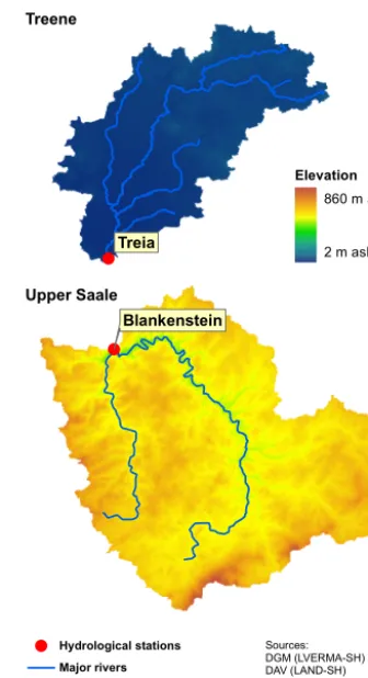
In contrasting catchments, different hydrological processes are of major relevance (Atkinson et al., 2002; Merz and Blöschl, 2004; Jothityangkoon and Sivapalan, 2009; Guse et al., 2016) and thus also the ability of a certain perfor-mance criterion in identifying a certain model parameter varies. With increasing relevance of a process, an accurate reproduction in the model becomes more important. There-fore, two catchments with different catchment characteristics were selected in this study to check the applicability of the proposed approach (Fig. 1). For the analysis, measured daily discharge time series from their catchment outlets were used to assess model performance.
2.1.1 Treene
The Treene catchment (up to the hydrological station Treia, 481 km2), located in northern Germany is a typical lowland catchment with strong groundwater dominance of total dis-charge even under high-flow conditions (Guse et al., 2014;
Treia
Elevation 860 m asl
2 m asl
Blankenstein
0 5 10 20
Kilometers
Hydrological stations Major rivers
Treene
Upper Saale
[image:3.612.341.509.66.375.2]Sources: DGM (LVERMA-SH) DAV (LAND-SH) River network (UBA) SRTM 90 (Jarvis et al., 2008)
Figure 1.Two study catchments (Treene and Saale) and their ment elevation. The same elevation legend is used for both catch-ments.
Pfannerstill et al., 2015; Guse et al., 2016). Moreover, tile flow is a relevant process since large parts of its agriculture area are drained (Kiesel et al., 2010). Other fast runoff com-ponents are of minor relevance as expected from the low to-pographic gradient in the catchment (maximum elevation of 80 m). The Treene catchment is dominated by agricultural ar-eas whilst only a minor part is covered by forests and urban areas (Guse et al., 2015). Mean annual precipitation is about 995 mm a−1with the highest values in summer months and monthly average temperature ranges from 1.5◦C (January) to 17.6◦C (July) with an average annual temperature of 9.2◦C.
Mean discharge at the catchment outlet is 6.23 m3s−1. 2.1.2 Upper Saale
catch-ment, the altitude in the Upper Saale catchment is higher (between 415 and 856 m) and slopes are steeper. Thus, fast runoff components are of higher relevance in this catchment. Mean annual precipitation is 929 mm a−1and monthly aver-age temperature ranges from −1.7◦C (January) to 17.2◦C (July) with an annual mean temperature of 7.9◦C. Mean dis-charge at the catchment outlet is 13.04 m3s−1.
2.2 Soil and Water Assessment Tool (SWAT)
The conceptual and process-based eco-hydrological model SWAT (Soil and Water Assessment Tool; Arnold et al., 1998) is used in this study. The SWAT model is spatially discre-tised into subbasins which are subdivided into hydrological response units (HRUs) based on unique underlying informa-tion on land use, soil and slope. All water balance compu-tations are conducted with daily temporal resolution at the scale of individual HRUs as the central calculation unit. The change in soil water storage is influenced by inputs (e.g. pre-cipitation) and outputs (e.g. evapotranspiration, runoff com-ponents).
In this study, the SWAT3S version (Pfannerstill et al., 2014a), which is a modification of the SWAT model, was used. In SWAT3S, the groundwater modelling has been im-proved by subdividing the active aquifer contributing to river discharge into a fast and a slow responding one. Different runoff components (surface runoff, lateral flow, groundwa-ter flow) are separately computed for each HRU and sum-marised as water yield of a subbasin. A detailed description of the SWAT model set-up for both catchments is described in Guse et al. (2016).
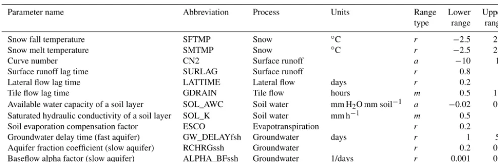
To analyse the relationship of performance criteria to model parameters, 12 SWAT model parameters from differ-ent hydrological compondiffer-ents which control differdiffer-ent parts of the hydrograph are selected in this study (Table 1). The fi-nal selection is based on studies with successful applications of the SWAT model within the studied catchments (Guse et al., 2016; Pfannerstill et al., 2015). Thus, parameter ranges were constrained according to authors’ previous knowledge with the aim of reducing unrealistic parameter combinations which may lead to physically implausible process descrip-tion.
Within the set of 12 parameters, 2 snow parameters reg-ulate snowfall and snowmelt. Infiltration and surface runoff are captured by CN2 which is included in the curve number approach (SCS, 1972). The timing of different runoff com-ponents within the land phase is represented by lag time rameters (SURLAG, LATTIME, GDRAIN). Three soil pa-rameters were included. For each soil layer, available water capacity (SOL_AWC) and saturated hydraulic conductivity (SOL_K) can be differentiated. The contribution of soil wa-ter from different soil depth for evaporation is regulated by a nonlinear function which is parameterised by ESCO. The groundwater module is parameterised with a retention time from soil to groundwater (GW_DELAYfsh), a partitioning
coefficient between the two aquifers (RCHRGssh) and the baseflow recession factor (ALPHA_BFssh).
Based on the physically meaningful selection of these 12 model parameters, their values were varied within a set of model simulations. The intention of these model simulations was to derive the interrelationship between model param-eters and performance criteria. For this, model simulations for the period from 2000 to 2010 were carried out based on 2000 different parameter sets that were generated with the latin hypercube sampling approach as implemented in the R package FME (Soetaert and Petzoldt, 2010). In the latin hypercube sampling, all model parameters were changed si-multaneously within the whole parameter space. For a more detailed description, readers are referred to Pfannerstill et al. (2014b).
All parameters values were already in a hydrologically plausible range according to prior modelling experience with the study sites. These constrained parameter ranges allowed for selecting an efficient but appropriate number of simula-tions to perform our analyses. Please note that the intention of the presented study was not to identify the parameter val-ues exactly, which allowed us to keep the sampling of the parameter space relatively sparse. Instead, we aimed to test and suggest the new connective strength approach. For this purpose, the number of 2000 model runs ensured a sufficient number of combinations at each node of the RTs.
2.3 Performance criteria
Ten performance criteria including five performance metrics and five signature measures were selected to capture differ-ent aspects of hydrological behaviour in models and as it was recommended in recent diagnostic model studies (Kling et al., 2012; Pechlivanidis et al., 2014; Pfannerstill et al., 2014b; Haas et al., 2016)
Nash–Sutcliffe efficiency (NSE) criterion (Eq. 1) is one of the most often used performance criteria in hydrology (Nash and Sutcliffe, 1970). NSE focuses on variability in measured discharge time series. It is known to give higher weights to high flows than to low flows (Schaefli and Gupta, 2007; Gupta et al., 2009; Pfannerstill et al., 2014b).
NSE=1− N
P
i=1
(Qo−Qs)2
N
P
i=1
(Qo−Qo)2
, (1)
whereQois measured discharge,Qsmodelled discharge and Qomean of measured discharge.
Table 1.List of SWAT models parameters. Lower and upper ranges are given as absolute range (r), additive (a) or multiplicative (m) value. Further information can be found in the theoretical documentation of the SWAT model (Neitsch et al., 2011).
Parameter name Abbreviation Process Units Range Lower Upper type range range Snow fall temperature SFTMP Snow ◦C r −2.5 2.5 Snow melt temperature SMTMP Snow ◦C r −2.5 2.5 Curve number CN2 Surface runoff a −10 10 Surface runoff lag time SURLAG Surface runoff r 0.8 4 Lateral flow lag time LATTIME Lateral flow days r 0.2 8 Tile flow lag time GDRAIN Tile flow hours m 0.5 1.5 Available water capacity of a soil layer SOL_AWC Soil water mm H2O mm soil−1 a −0.02 0.1 Saturated hydraulic conductivity of a soil layer SOL_K Soil water mm h−1 m 0.5 3 Soil evaporation compensation factor ESCO Evapotranspiration r 0.2 1 Groundwater delay time (fast aquifer) GW_DELAYfsh Groundwater days r 1 50 Aquifer fraction coefficient (slow aquifer) RCHRGssh Groundwater r 0.2 0.8 Baseflow alpha factor (slow aquifer) ALPHA_BFssh Groundwater 1/days r 0.001 0.2
time series. KGE_alpha is the variability ratio between the standard deviation of modelled (σs) and measured (σo)
dis-charge values. KGE_alpha larger than 1 shows that variabil-ity in modelled discharge time series is higher than in mea-sured discharge time series, while KGE_alpha lower than 1 represents the opposite case. KGE_beta is the bias ratio be-tween average values for modelled (µs) and measured (µo)
discharge. KGE_beta larger than 1 represents an overestima-tion of discharge, i.e. a positive bias, while values lower than 1 illustrate an underestimation. KGE_beta and KGE_alpha represent the reproduction of the first and the second mo-ments, respectively, as emphasised by Kling et al. (2012). KGE_r represents the correlation coefficient according to Pearson. KGE_r is used to analyse the agreement in tem-poral dynamics between measured and modelled discharge time series. To calculate KGE, the Euclidean distance to the ideal point in the 3-D criteria space which is created by its three components is calculated (Gupta et al., 2009). All three KGE components as well as KGE have an ideal value of one.
KGE= (2)
1−
q
(KGE_alpha−1)2+(KGE_beta−1)2+(KGE_r−1)2
KGE_alpha=σs/σo
KGE_beta=µs/µo
KGE_r=correlation coefficient
In addition to these five performance metrics, five signa-ture measures are selected based on FDC. The FDC only con-siders the discharge magnitude without considering the tem-poral occurrence of discharge values (Vogel and Fennessey, 1996; Yilmaz et al., 2008; Westerberg et al., 2011). To eval-uate the model performance, the FDC is subdivided into five FDC segments (very high, 0–5 % days of exceedance; high, 5–20 %; medium, 20–70 %; low, 70–95 %; very low, 95–100 %) as proposed by Pfannerstill et al. (2014b) and
evaluated separately. FDC signatures consider that different discharge magnitudes are controlled by different processes. Whilst the high-flow segment is mainly impacted by precip-itation and fast runoff components, low flows are controlled by evapotranspiration and deep groundwater storages (Yil-maz et al., 2008; Cheng et al., 2012; Pokhrel et al., 2012; Yaeger et al., 2012; Guse et al., 2016)
For the evaluation of each FDC segment, the RSR, the ra-tio of the root mean square error to the standard deviara-tion, was calculated for each FDC segment (Eq. 3) (Moriasi et al., 2007), which allows fair comparison between different seg-ments (Haas et al., 2016). The optimal value for RSR is 0. Using these five signature measures, the relation of model parameters to different discharge magnitudes can be derived (Pfannerstill et al., 2014b; Guse et al., 2016).
RSR=
s 1
N N
P
i=1
(Qo−Qs)2
s 1
N N
P
i=1
(Qo−Qo)2
(3)
These 10 different performance criteria were calculated for all 2000 simulation runs. Both parameter sets and calculated performance criteria from these simulations were then used for the following analyses.
2.4 Regression trees
Regression trees (RTs) are a method used to order the re-lationship between several explaining variables and a single target variable (Breiman et al., 1984). It is a binary algorithm based on logical expressions. In a sequence of regressions, the explaining variable is subsequently determined from a set of variables that has the highest predictive value for the target variable being analysed. At each node of a regression tree, the (sub)set of model simulations is subdivided into two subsets based on a threshold value for one of the explaining variables (Singh et al., 2014a, b). All simulations with a value in the explaining variable above the threshold belong to the one group, and those with a value below the threshold to the other group. For each node, this approach is repeated until no further subdivision of a variable at a certain node explains the target variable.
The sequence of decisions is visualised in a tree diagram to detect the importance of different explaining variables for the target variable. A regression tree consists of multiple branches. Either a different or an already chosen explaining variable is selected in the next branch of the tree. The com-plexity of the tree reflects the comcom-plexity of the relationship between explaining and target variables.
The earlier a variable is used in the construction of an RT, the higher its importance is. The variable used in the first split has thus the maximum importance. The gain in information is maximised by defining clearly separated subgroups of the whole simulation set (Singh et al., 2014b).
For our analyses, we used the R package rpart (Therneau et al., 2015). In the rpart package, the contribution of each explaining variable on changes in the target variable is calcu-lated. The variable importance describes how the prediction is reduced when removing this explaining variable. Thus, it summarises the contribution of the explaining variables in all nodes in explaining the changes in the target variable.
Thus, it is considered both that the explaining variable can be the most important one (and thus defines the subdivision of the subset) and that a variable has lower explanation power than the primary variable and is thus not shown in the trees. Thus, explaining variables that are not shown in the tree can also have a relevant value of variable importance. The per-centage contribution of each explaining variable shows its importance for the target variable (Singh et al., 2014b). 2.4.1 Regression trees using performance criteria as
target variables (RTperf)
RTs are applied in this study in two approaches using 2000 model simulations with pre-selected model parameters and calculated performance criterion. In our case, the set of 2000 parameter sets and performance criteria are large enough to ensure a sufficient number of combinations at each node of RT. In the first application the selected 10 performance cri-teria are used consecutively as target variables to construct
regression trees for each performance criterion (named RT-perf). As explaining variables, model parameters are used to detect which of them lead to changes in a performance crite-rion. The relevance of each model parameter is derived from regression trees by calculating the percentage contribution of each model parameter in explaining the variability in a per-formance criterion. This leads to identification of the most relevant model parameters for each performance criterion. 2.4.2 Regression trees using model parameters as
target variables (RTpar)
Furthermore, we aim to detect more than the most relevant parameters for a certain performance criterion. Thus, in the second application, the importance of performance criteria which are most strongly impacted by changes in the value of a certain parameter is identified. This cannot be derived from RTperf. To achieve this, a bijective approach is required by looking from the point of model parameters.
Thus, this step was initialised in the opposite way to RT-perf to analyse how changes in model parameters influence performance criteria. To achieve this, explaining and target variables in RT are permuted. Each model parameter is used as the target variable in RT and all performance criteria as explaining variables (named RTpar). In RTpar model param-eters are analysed individually. Similarly to RTperf, the per-centage contribution of each performance criterion is calcu-lated to explain the impact of changes in values of a certain model parameter.
2.4.3 Connective strength by comparing both regression tree approaches
A core advantage of RT is that subsets of simulation runs are constructed in a structured way. By subdividing the sim-ulation set based on the major influencing variables at each branch, two distinct subsets occur which differ with respect to values of model parameters as well as with respect to per-formance criteria. With this subset construction, the model parameter or performance criteria which has the highest ex-planatory power in an RT branch can be detected. This allows for a bijective analysis of the relationship between model pa-rameters and performance criteria.
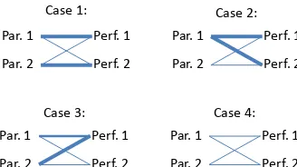
In addition to RTperf and RTpar, the percentage contri-butions as derived from both RT approaches are compared to analyse the connective strength between model parame-ters and performance criteria. Thus, four cases of connective strength for each pair of model parameter and performance criterion can be differentiated (Fig. 2).
Par. 1
Par. 2
Perf. 1
Perf. 2 Case 1:
Par. 1
Par. 2
Perf. 1
Perf. 2 Case 2:
Par. 1
Par. 2
Perf. 1
Perf. 2 Case 3:
Par. 1
Par. 2
Perf. 1
[image:7.612.86.250.65.157.2]Perf. 2 Case 4:
Figure 2.Chart of four cases of connective strength between model parameters and performance measures. A thicker blue line shows a higher impact of the model parameter on the performance criteria
optimal case representing a high connective strength and occurs if a certain parameter influences one per-formance criterion to a large extent without influencing other performance criteria significantly.
2. High percentage contribution in RTperf, but low in RT-par: in this case, a certain model parameter controls the selected performance criterion. However, this model pa-rameter also influences other performance criteria. This case occurs if the corresponding hydrological compo-nent is very dominant and influences multiple perfor-mance criteria. Here, the connective strength cannot be fully understood when using performance criteria as tar-get variables. From the side of the model parameter, further investigation is required regarding which perfor-mance criterion is most appropriate for parameter iden-tification.
3. Low percentage contribution in RTperf, but high in RT-par: in this case, the model parameter is not the ma-jor controlling parameter on the selected performance criterion as detected in RTperf. However, its impact on other performance criteria is even lower which results in a high value in RTpar. Thus, the selected performance criterion is appropriate to explain the impact of changes in this model parameter, but the performance criterion is even more strongly impacted by other model parame-ters. This case occurs if the corresponding hydrological component is of minor relevance in describing the hy-drological system of the catchment. Thus, due to its low relevance, the connective strength is also low and a pa-rameter identification is not precise.
4. Low percentage contributions in both RTs: in this case, this model parameter does not impact the performance criterion to a relevant extent, nor is the performance cri-terion impacted by changes in the parameter. Thus, the connective strength is low. This parameter is not identi-fiable due to low relevance of the corresponding hydro-logical component and no distinct relationship with one of the performance criteria.
By applying this approach in two catchments with differ-ent characteristics, we analyse how strongly a certain perfor-mance criterion is connected to a specific model parameter and how this connective strength depends on the relevance of the corresponding hydrological component.
3 Results
3.1 Correlation between performance criteria
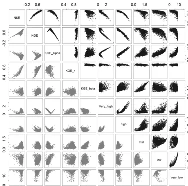
In order to understand similarities of performance criteria, pairwise correlation analysis of all performance criteria is carried out separately for each catchment. In the Treene catchment (Fig. 3, upper panel), NSE, KGE and RSR of very high and high segments of FDC are strongly correlated. Moreover, RSR of low and very low flows are highly corre-lated. KGE is mainly controlled by its variability component (KGE_alpha) meaning that good performance of KGE_alpha (optimum=1) also results in high performance in KGE. KGE_beta (bias component) is correlated with the middle segment of FDC. Concerning values of the performance cri-teria, KGE_alpha and KGE_beta are mostly higher than one, indicating an overestimation and higher variability in mod-elled discharge than in the measured one. Good performance in a certain segment of FDC occurs in the case of good formance in the adjacent segment(s). In the case of good per-formance for low flows, very low flows also perform well. Similarly, good performance for very high flows was also detected in model runs with good performance in high flows. However, correlations between RSR of (very) high and (very) low flows are lower which indicates that there are less model runs with good performance in both high and low flows.
Figure 3.Scatter plot matrix of performance criteria of Treene (in black,a) and Saale (in grey,b) catchment showing pairwise performance criteria plots for 2000 model simulations. The scales on the sides show values of the respective performance criterion.
3.2 Impact of model parameters on performance criteria (RTperf)
The connective strength between model parameters and per-formance criteria was investigated using regression trees (RTs). At first, RTs were constructed using the 10 perfor-mance criteria (RTperf) as target variables. The aim of this step was to detect which model parameter most strongly af-fects a certain performance criterion.
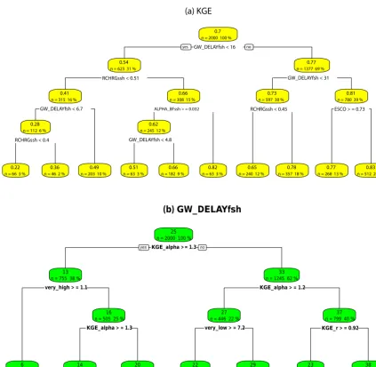
Figure 4 shows the regression tree for KGE for the Treene catchment exemplarily for RTperf. Looking from top down, the most influencing model parameters for KGE are pro-vided. The first branch is defined by groundwater retention time of the first aquifer (GW_DELAYfsh) and the second one on the right side again by GW_DELAYfsh and on the left side by the aquifer partitioning coefficient (RCHRGssh). In total, only groundwater parameters affect KGE to a relevant extent. When going along the right side of the branch, pa-rameter settings of the controlling model papa-rameter at these
nodes are identified which lead to the best KGE on average (0.83).
KGE
KGE KGE KGE KGE KGE KGE (a) KGE
GW_DELAYfsh < 16
RCHRGssh < 0.51
GW_DELAYfsh < 6.7
RCHRGssh < 0.4
ALPHA_BFssh > = 0.032
GW_DELAYfsh < 4.8
GW_DELAYfsh < 31
RCHRGssh < 0.45 ESCO > = 0.73 0.7
n = 2000 100 %
0.54
n = 623 31 %
0.41
n = 315 16 %
0.28
n = 112 6 %
0.22
n = 66 3 %
0.36
n = 46 2 %
0.49
n = 203 10 %
0.66
n = 308 15 %
0.62
n = 245 12 %
0.51
n = 63 3 %
0.66
n = 182 9 %
0.82
n = 63 3 %
0.77
n = 1377 69 %
0.73
n = 597 30 %
0.65
n = 240 12 %
0.78
n = 357 18 %
0.81
n = 780 39 %
0.77
n = 268 13 %
0.83
n = 512 26 %
yes no
GW_DELAYfshGW_DELAYfshGW_DELAYfshGW_DELAYfshGW_DELAYfshGW_DELAYfsh (b) GW_DELAYfsh
KGE_alpha > = 1.3
very_high > = 1.1
KGE_alpha > = 1.3
KGE_alpha > = 1.2
very_low > = 7.2 KGE_r > = 0.92 25
n = 2000 100 %
13 n = 755 38 %
6 n = 250 12 %
16 n = 505 25 %
14 n = 306 15 %
20 n = 199 10 %
33 n = 1245 62 %
27 n = 446 22 %
22 n = 110 6 %
29 n = 336 17 %
37 n = 799 40 %
23 n = 48 2 %
38 n = 751 38 %
[image:9.612.87.510.62.474.2]yes no
Figure 4.Example of a regression tree (RT) using(a)KGE as the target variable and model parameters as explaining variables and(b)the model parameter GW_DELAYfsh as the target variable and performance criteria as explaining variables for the Treene catchment.
controlled by the baseflow recession coefficient of the second aquifer (ALPHA_BFssh) in addition to GW_DELAYfsh. Seven of twelve model parameters, namely fast runoff (CN2, SURLAG, GDRAIN, LATTIME), soil (SOL_K) and snow parameters (SFTMP, SMTMP), have only a minor impact on all performance criteria and cannot be identified by the se-lected performance criterion.
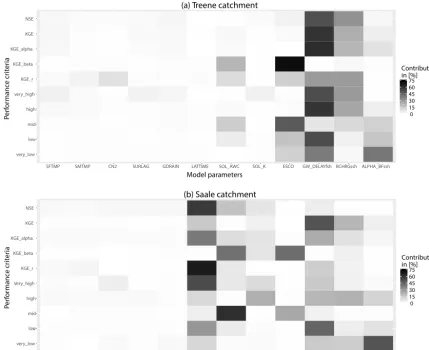
Figure 5 shows that the relationship between model pa-rameters and performance criteria is more complex in the Saale catchment compared to the Treene catchment. A clear classification into groups of performance criteria which are controlled by certain model parameters is more difficult. Four performance criteria (NSE, KGE_alpha, KGE_r, very high-flow segment of FDC) are controlled by lateral high-flow lag time (LATTIME). But these performance criteria are also influenced by groundwater parameters (GW_DELAYfsh,
RCHRGssh). Furthermore, RSR for high flows is not con-trolled by LATTIME but by these two groundwater param-eters and hydraulic conductivity in soil (SOL_K). KGE is controlled by a parameter (GW_DELAYfsh) which does not have the largest percentage contribution for one of its three components. Water balance (KGE_beta) is controlled by ESCO and SOL_AWC, while mid-flows are mainly influenced by SOL_AWC. Low flows are controlled by GW_DELAYfsh and very low flows by ALPHA_BFssh. Snow and fast runoff parameters except LATTIME do not influence any of the performance criteria to a great extent. Thus, parameters exist without significant impact and LAT-TIME controls multiple performance criteria in the Saale catchment as well.
very_low low mid high very_high KGE_r KGE_beta KGE_alpha KGE NSE
SFTMP SMTMP CN2 SURLAG GDRAIN LATTIME SOL_AWC SOL_K ESCO GW_DELAYfsh RCHRGssh ALPHA_BFssh
Model parameters
Perf
or
mance cr
iter
ia
0 15 30 45 60 75 Contribution in [%]
(a) Treene catchment
very_low
low
mid high Very_high KGE_r KGE_beta KGE_alpha KGE NSE
SFTMP SMTMP CN2 SURLAG GDRAIN LATTIME SOL_AWC SOL_K ESCO GW_DELAYfsh RCHRGssh ALPHA_BFssh
Model parameters
Perf
or
mance cr
iter
ia
0 15 30 45 60 75 Contribution in [%]
[image:10.612.85.515.68.418.2](b) Saale catchment
Figure 5.Regression trees (RTs) using performance criteria as target variables. The percentage contribution of model parameters in explain-ing performance criteria is shown for Treene(a)and Saale(b)catchment. In every row the percentage contributions sum up to 100 %.
performance criteria are found for several model parame-ters (e.g. CN2), which shows the low connective strength between these model parameters and performance criteria. This leads to more challenging identification of parameter values. It is important to detect whether the low relevance of a model parameter is related to the minor relevance of the corresponding process or whether the selected performance criterion is inappropriate to identify this model parameter. Moreover, some model parameters highly influence multiple performance criteria (e.g. GW_DELAYfsh and RCHRGssh in the Treene, LATTIME in the Saale), which leads to unclear results in the connective strength between model parameters and performance criteria. This suggests that these parameters govern the overall hydrological system in the model.
3.3 Impact of changes in model parameters on performance criteria (RTpar)
In the second RT application, the roles of model parameters and performance criteria are permuted. The relationship
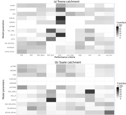
be-tween model parameters and performance criteria is analysed using 12 model parameters consecutively as target variables. It is investigated which performance criteria are impacted by changes in model parameters (RTpar, Fig. 6).
ALPHA_BFssh RCHRGssh GW_DELAYfsh ESCO SOL_K SOL_AWC LATTIME GDRAIN SURLAG CN2 SMTMP SFTMP
NSE KGE KGE_alpha KGE_beta KGE_r very_high high mid low very_low
Performance criteria
Model par
ameters
0 15 30 45 60 75
Contribution in [%] (a) Treene catchment
ALPHA_BFssh RCHRGssh GW_DELAYfsh ESCO SOL_K SOL_AWC LATTIME GDRAIN SURLAG CN2 SMTMP SFTMP
NSE KGE KGE_alpha KGE_beta KGE_r very_high high mid low very_low
Performance criteria
Model par
ameters
0 15 30 45 60 75
Contribution in [%]
[image:11.612.82.513.68.463.2](b) Saale catchment
Figure 6.Regression trees (RTs) using model parameters as target variables (RTpar) for Treene(a)and Saale(b)catchment and performance criteria as explaining variables. All values of a parameter are in white in the case that the resulting variation among performance criteria for this parameter was too low to construct a regression tree. In every row the percentage contributions sum up to 100 %.
model component, SOL_AWC and ESCO are strongly re-lated to water balance (KGE_beta) and to a lower extent to RSR for mid-flows. ALPHA_BFssh is related to RSR of low and very low flows as well as to NSE. For the two groundwa-ter paramegroundwa-ters (GW_DELAYfsh, RCHRGssh), four perfor-mance criteria (NSE, KGE, KGE_alpha, RSR for high flows) have a similar percentage contribution. This point shows that both groundwater parameters control different aspects of hy-drological model behaviour without having a clear relation-ship with a certain part of the hydrograph.
In the Saale catchment (Fig. 6), snow parameters (SFTMP, SMTMP) and LATTIME affect both KGE_r and NSE. Changes in curve number (CN2) mainly influence KGE_alpha and RSR for very high flows. Thus, variability between measured and modelled discharge time series and in particular high flows are influenced by CN2. All three soil
parameters (SOL_AWC, SOL_K, ESCO) influence water balance (KGE_beta) and mid-flow segment of FDC. How-ever, evaporation (ESCO) is more related to KGE_beta while SOL_AWC has the largest impact on mid-flows. In the case of GW_DELAYfsh several performance criteria are affected to a similar extent, but none of them has a high percentage contribution. While RCHRGssh affects KGE and high flows, ALPHA_BFssh strongly controls very low flows.
3.4 Comparing RTperf and RTpar
● ● ● ● ● ● ● ● ● ● ●
0 20 40 60 80
0 20 40 60 80 NSE
RCHRGssh●GW_DELAYfsh LATTIME ● ● ● ● ● ● ● ● ● ● ● ●
0 20 40 60 80
0 20 40 60 80 KGE GW_DELAYfsh RCHRGssh GW_DELAYfsh RCHRGssh ● ● ● ● ● ●● ● ● ● ● ●
0 20 40 60 80
0 20 40 60 80 KGE_alpha GW_DELAYfsh LATTIME RCHRGssh GW_DELAYfsh ● ● ● ● ● ● ● ● ● ●●●
0 20 40 60 80
0 20 40 60 80 KGE_beta SOL_AWC ESCO SOL_AWC ESCO ● ● ● ● ● ● ● ● ● ● ● ●
0 20 40 60 80
0 20 40 60 80 KGE_r SMTMP SURLAG GDRAIN SOL_K GW_DELAYfsh RCHRGssh LATTIME ● ● ● ● ● ●● ●● ● ● ●
0 20 40 60 80
0 20 40 60 80 very_high GW_DELAYfsh
RCHRGssh LATTIME ●
● ● ●● ● ● ●● ● ● ●
0 20 40 60 80
0 20 40 60 80 high GW_DELAYfsh RCHRGssh RCHRGssh SOL_K ● ● ● ● ● ● ● ● ● ● ● ●
0 20 40 60 80
0 20 40 60 80 mid SOL_AWC ESCO SOL_AWC ESCO ● ● ● ● ● ●● ● ● ● ● ●
0 20 40 60 80
0 20 40 60 80 low GW_DELAYfsh LATTIME GW_DELAYfsh ● ● ● ●● ● ●● ● ● ● ●
0 20 40 60 80
[image:12.612.51.547.65.260.2]0 20 40 60 80 very_low ALPHA_BFssh GW_DELAYfsh GW_DELAYfsh ALPHA_BFssh RTperf R Tpar
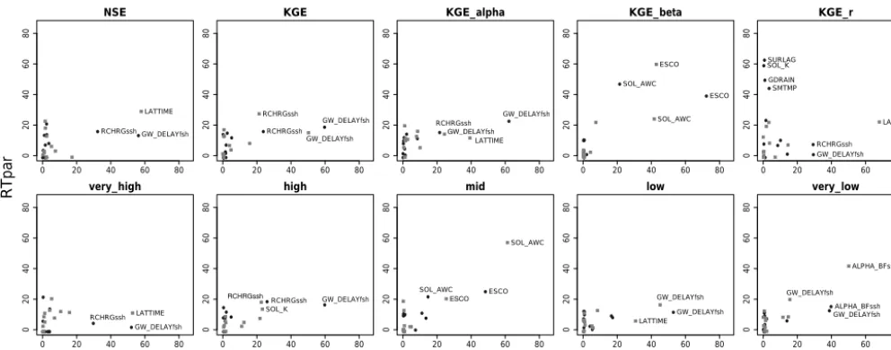
Figure 7.Connective strength between performance criteria and model parameters. The percent contribution of pairs of model parameter and performance criterion are shown as derived from RTperf (xaxis) and RTpar (yaxis). A high value along thexaxis shows a high contribution of a model parameter in explaining variability in the performance criterion as detected by RTperf. A high value along theyaxis (RTpar) shows that this performance criterion is most strongly impacted among all performance criteria by changes in the model parameter. Strong connective strength is detected if both values are high. The pairs with at least one high-percentage contribution are labelled. The results from Treene catchment are shown as black circles and from Saale catchment in grey squares. Please note that percentage contributions on thex axis sum up to 100 %, while this is not the case for theyaxis.
model parameter and performance criteria. A high connec-tive strength between a distinct model parameter and a dis-tinct performance criterion is given if (1) the model param-eter is one of the dominant controls for the performance cri-terion and (2) the same performance cricri-terion is sensitive to changes in the model parameter values to a relevant extent.
For mid-and low-flow conditions, both RTperf and RTpar provide strong connective strength with high percentage con-tribution in RTperf and RTpar for the same pair of model parameter and performance criterion in both catchments. The strong relationship of evaporation (ESCO) and available soil water capacity (SOL_AWC) to RSR of mid-flows and KGE_beta is derived in both RT approaches (Fig. 7). Wa-ter balance (KGE_beta) is hereby more controlled by ESCO, whilst SOL_AWC is the dominant parameter for mid-flows especially in the Saale catchment.
Similarly, the connection between RSR for the very low segment of FDC and the baseflow recession coefficient (AL-PHA_BFssh) is strong particularly in the Saale catchment. In both catchments the retention time of recharge into ground-water (GW_DELAYfsh) is also relevant.
KGE is dominated by GW_DELAYfsh and the aquifer partitioning coefficient (RCHRGssh) in a similar way in both catchments despite contrasting catchment characteristics. In RTperf, KGE is most strongly impacted by GW_DELAYfsh. However, in RTpar, KGE has a higher percentage con-tribution in explaining changes in RCHRGssh than in GW_DELAYfsh.
A very specific pattern is detected for KGE_r in the Treene catchment. In RTpar, a high percentage contribution of KGE_r for model parameters of lower relevance is de-tected. High values for RTpar and low values for RTperf in Fig. 7 show that KGE_r is the most appropriate performance criterion to assess changes in these model parameters. How-ever, due to low relevance of snow or surface runoff, KGE_r is controlled by groundwater parameters. Here, we see a large difference in the interrelationship between model parameters and performance criteria by comparing RTperf and RTpar.
4 Discussion
The aim of this study was to improve the understanding of the relationship between model parameters and performance cri-teria. To this end, the concept of connective strength between model parameters and performance criteria was introduced, based on two approaches of regression trees first using per-formance criteria and then model parameters as target vari-ables. Based on this, we discuss how the connective strength to the performance criteria varies between different model parameters and how the use of different performance criteria help in identifying model parameters.
4.1 Benefit of analysing bijectively the relationship between model parameters and performance criteria
By analysing the connective strength, the performance crite-ria which are appropcrite-riate to best constrain the model param-eters are identified. The novelty of this study lies in the as-sessment of the relationship between model parameters and performance criteria bijectively (RTperf, RTpar).
In RTperf, detection for 10 performance criteria is per-formed to ascertain whether the same model parameters af-fect different performance criteria. It is shown that not all model parameters influence one of the selected performance criteria (see Fig. 5). This indicates that not all model pa-rameters can be identified with this approach since either the model parameters are not relevant or appropriate perfor-mance criteria are still missing to describe the changes in this model parameter. The impact of model parameters on perfor-mance criteria depends on the relevance of the correspond-ing process. In the case that the relevance of the associated process is very low, parameters from other more dominant processes control performance criteria. This is for example shown for curve number (CN2). Its impact on performance criteria in Treene catchment is low due to higher contribution of groundwater flow compared to surface runoff.
In RTpar with model parameters as target variables, each model parameter is individually assessed. By comparing RT-par for different model RT-parameters, the influence of model parameters on different performance criteria is identified. It can be derived whether parameters and their associated
pro-cesses are of low relevance or whether an appropriate perfor-mance criterion for a model parameter is missing. The RTpar approach shows for the majority of the model parameters that changes in their values are detectable at least by one selected performance criteria. This indicates that the impact of model parameters related to processes of minor relevance on perfor-mance criteria can be derived with RTpar.
Differences between RTperf and RTpar are also obtained for parameters related to the most dominant process(es). The groundwater parameters (mainly GW_DELAYfsh) con-trol most of performance criteria for the Treene catchment (Fig. 5). A similar result is obtained for the Saale catchment with a dominance of lateral flow lag time (LATTIME). Com-paring results of two RT approaches, a higher similarity be-tween both catchments is detected in RTpar (Fig. 6).
Comparing the results of both RT approaches (Figs. 5 and 6), it becomes apparent that the performance criterion with the highest percent contribution for a given model parameter in Fig. 5 is in some cases not identical with the performance criterion with highest percent contribution in Fig. 6. Thus, the analysis from the side of the model parameters provides addi-tional information about the interrelationship between model parameters and performance criteria.
The interpretation of the relationship between model pa-rameters and performance criteria from both sites by means of the suggested connective strength extends the classical one-sided analysis of the impact of model parameters on per-formance criteria as in, for example, sensitivity analyses (van Werkhoven et al., 2008; Herman et al., 2013). In our ap-proach both performance criteria and model parameters were analysed separately as target variables. In comparison to the established one-sided approaches, this yields additional in-formation on which performance criteria are appropriate for a certain model parameter.
Thus, we investigate not only how variations are prop-agated in the model up to the output but also which out-puts (i.e. performance criteria) are impacted by a certain model parameter. The comparison of parameter relevance with former studies on temporally resolved parameter sensi-tivity analyses (Guse et al., 2014, 2016) shows that the over-all ranking of model parameters is similar.
can be clearly related to a specific part of hydrological be-haviour (Kling et al., 2012), the RT shows whether a model parameter is more relevant in representing variability, bias or correlation in modelled discharge time series. By compar-ing the performance in KGE with its components, the most important aspect in evaluating the model performance with KGE becomes apparent. For example, in the Treene catch-ment variability is the most important one, as indicated by KGE_alpha.
The differences in pairwise correlations of performance criteria between both catchments also result in differences in the relationship between model parameters and a certain performance criterion. Similar results in KGE and NSE are calculated in the case of high correlation between KGE and KGE_alpha and thus the most relevant model parameters on these two performance criteria are similar. The opposite re-sult is obtained in the Saale catchment. Due to low values of KGE_alpha, different parameters control KGE and NSE. This pattern is reasonable since both KGE_alpha and NSE focus on assessment of variability in discharge time series, while the three components (variability, bias, correlation) are equally weighted in KGE.
Concerning signature measures, this study shows that dif-ferent parameters are related to FDC segments. This is in line with studies stating that each FDC segment can be related to certain catchment processes (Yilmaz et al., 2008; Yaeger et al., 2012; Pfannerstill et al., 2015). The strong connec-tive strength of model parameters regulating water balance to mid-flows as well as of parameters from slow reacting aquifer storages to very low flows is derived in this study. However, a typical sequence of a high connective strength of high flows to surface runoff parameters is not identified. Moreover, we observe that dominant processes, i.e. ground-water flow in the Treene and lateral flow in the Saale catch-ment, influence both high and low flows. This leads to a trade-off in parameter identification since the same model parameters control high and low flows. This shows that per-formance criteria should be specific for different model pa-rameters, in this case specific for either high or low flow, to avoid a high parameter uncertainty and equifinality in the es-timation of behavioural parameter sets.
4.3 Number of required performance criteria
The analysis of the bijective connective strength between pairs of model parameters and performance criteria in the two catchments shows that the most appropriate performance criterion varies depending on different model parameters. Pairs with a high connective strength were detected and grouped. This results in a minimum number of three re-quired performance criteria related to high-, mid- and low-flow conditions since the most relevant parameters between these three types of performance criteria vary. This is in line with other studies on performance criteria stating that three or four performance criteria are needed at a minimum to
cap-turing different parts of the hydrological system (Madsen, 2000; Boyle et al., 2001; van Werkhoven et al., 2008, 2009). In addition, an individual performance criterion for a sin-gle model parameter might be needed, e.g. to assess the importance of mid-flows (van Werkhoven et al., 2008; Wa-gener et al., 2009; Herman et al., 2013). This is shown in the RT analysis, where the controlling parameters for KGE_beta and RSR for mid-flows are different compared to other per-formance criteria and these dominant model parameters are from soil components and related to water balance. In these cases, the connective strength is very high.
In addition, for the assessment of low-flow conditions, an individual performance criterion is needed which was in this case RSR for low and very low flows. A high connective strength between model parameter and performance criterion was detected for very low flows. Moreover, the requirement for a segmentation of FDC into very low and low flows as in-troduced by Pfannerstill et al. (2014b) is emphasised by iden-tifying different relevant model parameters. The high corre-lation between RSR for very low and low flows in the Treene catchment also results in similar dominant parameters, while different parameters control these signature measures in the Saale catchment (see Fig. 5). Thus, similar influencing pa-rameters in RTperf for different performance criteria are de-tected if both are highly correlated.
High flows are driven by interacting and overlaying pro-cesses from different hydrological components. Here, the most influential parameters and the most appropriate perfor-mance criterion vary depending on the type of errors which are dominant in the modelling process. The complexity in the representation of high flows depends on the involved processes. In the groundwater-dominated Treene catchment, the RT analysis for five performance criteria related to high flows provides very similar results. The RT analysis using model parameters as explaining variables (RTpar) however highlights differences in the relationship of model parame-ters and these five performance criteria. In the Saale catch-ment, relevant model parameters largely vary between all performance criteria related to high flows. Here, all selected performance criteria capture different types of errors in mod-elled discharge time series. The analysis of deviations be-tween measured and modelled discharge in this catchment is more complex so that more than one performance criterion for high flows is required. With higher heterogeneity in dom-inant processes and strong interaction of different processes in controlling hydrological behaviour, a more distinct selec-tion of a larger set of performance measures is required.
As demonstrated in this study, the results vary between dif-ferent catchments. Further studies in other catchments might additionally improve the understanding of the connective strength between model parameters and performance crite-ria using this methodology. A separate approach for specific time periods, for example, in winter to capture the impact of snow parameters, might be an upcoming interest. Due to the generality of the suggested approach, applicability with other models is expected.
5 Conclusion
For achieving precise parameter identification, the connec-tive strength between model parameters and different per-formance criteria is analysed. For this, two regression tree (RT) approaches are applied using consecutively perfor-mance criteria and model parameters as target variables. This method derives which model parameters affect a per-formance criterion (RTperf) and which perper-formance crite-ria are impacted by changes in model parameters (RTpar). By detecting the connective strength between model param-eters and performance criteria, appropriate performance cri-teria can be derived for different model parameters. Based on precise parameter identification and a better understanding of model parameters, parameter uncertainty and thus equifinal-ity among different model runs can be reduced.
Thus, the main outcomes of this study are as follows: 1. The pairwise correlation between performance criteria
varies between the two catchments depending on the model error. Thus, different performance criteria are re-quired to disentangle the impact of different hydrolog-ical behaviour on modelled discharge. The number of required performance criteria is higher for catchments with a higher process complexity.
2. In RTperf, it becomes apparent how largely the rele-vance of model parameters varies between different per-formance criteria. Our study emphasises the importance of a separate consideration of KGE components and of a signature-based analysis of different FDC segments for precise parameter identification. Differences in domi-nant parameters are detected between performance cri-teria related to high-, mid- or low-flow conditions. 3. RTpar, which uses model parameters as target
vari-ables, shows which performance criterion is appropri-ate to identify a model parameter. Similar results in RT-perf and RTpar demonstrate high capability of a per-formance criterion to consider the impact of a model parameter accurately. Contrasting results are in particu-lar derived for model parameters which are related to processes of minor relevance. A bijective connective strength between model parameters and performance criteria is detected for low and mid-flows, whilst mod-elling of high flows is more complex both in terms of
relevant model parameters and appropriate performance criteria.
Overall, this study shows that multiple performance crite-ria are required for accurate parameter identification for re-liable hydrological modelling. However, no general conclu-sion regarding universal performance criteria can be drawn, since the connective strength between model parameters and performance criteria varies between catchments depending on hydrological complexity of the catchments with respect to processes and their relevance in controlling hydrological behaviour in models. Using the presented approach, one can derive how precisely reasonable values of model parameters can be identified by a set of performance criteria.
Data availability. We are not permitted to distribute all data of the hydrological model. The results of the model simulations can be provided upon request by contacting the first author.
Competing interests. The authors declare that they have no conflict of interest.
Acknowledgements. We thank the DFG for financially supporting the first author (BG; project GU 1466/1-1 Hydrological consistency in modelling). Furthermore we thank the CAWa (Central Asian Water) project (www.cawa-project.net, contract no. AA7090002) of the German Federal Foreign Office as part of the German Wa-ter Initiative for Central Asia (Berlin Process) for the funding of the third author (AG). The fourth author (JK) was funded through the GLANCE project (Global change effects in river ecosystems; 01LN1320A) supported by the German Federal Ministry of Educa-tion and Research (BMBF). The fifth author (CL) received funding from the Leibniz Association (SAW-2012-IGB-4167) within the In-ternational Leibniz Research School: Aquatic boundaries and link-ages in a changing environment (Aqualink).
We thank the Agency for Coastal Defence, National Park and Marine Conservation of Schleswig–Holstein (LKN-SH) and the State Institute for Environment and Geology of Thuringia (TLUG) for the discharge data. We thank Martin Volk and Michael Strauch (UFZ) for contributing to the SWAT modelling in the Saale catch-ment. Furthermore, we thank the community of the open-source software R, which we used for this study.
Edited by: Dimitri Solomatine
References
Abebe, N. A., Ogden, F. L., and Pradhan, N. R.: Sensitivity and un-certainty analysis of the conceptual HBV rainfall-runoff model: Implications for parameter estimation, J. Hydrol., 389, 301–310, 2010.
Arnold, J. G., Srinivasan, R., Muttiah, R. S., and Williams, J. R.: Large area hydrologic modeling and assessment part I: model development, J. Am. Water Resour. As., 34, 73–89, 1998. Atkinson, S. E., Woods, R. A., and Sivapalan, M.: Climate
and landscape controls on water balance model complex-ity over changing timescales, Water Resour. Res., 38, 1314, https://doi.org/10.1029/2002WR001487, 2002.
Boyle, D. P., Gupta, H. V., Sorooshian, S., Koren, V., Zhang, Z., and Smith, M.: Toward improved streamflow forecasts: Value of semidistributed modeling, Water Resour. Res., 37, 2749–2759, 2001.
Breiman, L., Friedman, J. H., Olshen, R. A., and Stone, C. J.: Classi-fication and Regression Trees, CRC Press, Wadsworth, Belmont, CA, 1984.
Cheng, L., Yaeger, M., Viglione, A., Coopersmith, E., Ye, S., and Sivapalan, M.: Exploring the physical controls of re-gional patterns of flow duration curves – Part 1: Insights from statistical analyses, Hydrol. Earth Syst. Sci., 16, 4435–4446, https://doi.org/10.5194/hess-16-4435-2012, 2012.
Euser, T., Winsemius, H. C., Hrachowitz, M., Fenicia, F., Uhlen-brook, S., and Savenije, H. H. G.: A framework to assess the re-alism of model structures using hydrological signatures, Hydrol. Earth Syst. Sci., 17, 1893–1912, https://doi.org/10.5194/hess-17-1893-2013, 2013.
Fenicia, F., Savenije, H. H., Matgen, P., and Pfister, L.: A comparison of alternative multiobjective calibration strategies for hydrological modeling, Water Resour. Res., 43, W03434, https://doi.org/10.1029/2006WR005098, 2007.
Gupta, H. V., Wagener, T., and Liu, Y.: Reconciling theory with observations: Elements of a diagnostic approach to model evalu-ation, Hydrol. Process., 22, 3802–3813, 2008.
Gupta, H. V., Kling, H., Yilmaz, K. K., and Martinez, G. F.: Decom-position of the mean squared error and NSE performance criteria: Implications for improving hydrological modelling, J. Hydrol., 377, 80–91, 2009.
Gupta, H. V., Sorooshian, S., and Yapo, P. O.: Toward improved cal-ibration of hydrologic models: Combining the strengths of man-ual and automatic methods, Water Resour. Res., 34, 751–763, 1998.
Gupta, H. V., Perrin, C., Blöschl, G., Montanari, A., Kumar, R., Clark, M., and Andréassian, V.: Large-sample hydrology: a need to balance depth with breadth, Hydrol. Earth Syst. Sci., 18, 463– 477, https://doi.org/10.5194/hess-18-463-2014, 2014.
Guse, B., Reusser, D. E., and Fohrer, N.: How to improve the representation of hydrological processes in SWAT for a low-land catchment – temporal analysis of parameter sensitiv-ity and model performance, Hydrol. Process., 28, 2651–2670, https://doi.org/10.1002/hyp.9777, 2014.
Guse, B., Pfannerstill, M., and Fohrer, N.: Dynamic modelling of land use change impacts on nitrate loads in rivers, Environ. Process., 2, 575–592, https://doi.org/10.1007/s40710-015-0099-x, 2015.
Guse, B., Pfannerstill, M., Strauch, M., Reusser, D. E., Volk, M., Gupta, H. V., and Fohrer, N.: On characterizing the temporal
dominance patterns of model parameters and processes, Hydrol. Process., 30, 2255–2270, https://doi.org/10.1002/hyp.10764, 2016.
Haas, M. B., Guse, B., Pfannerstill, M., and Fohrer, N.: A joined multi-metric calibration of river discharge and nitrate loads with different performance measures, J. Hydrol., 536, 534–545, https://doi.org/10.1016/j.jhydrol.2016.03.001, 2016.
Herman, J. D., Reed, P. M., and Wagener, T.: Time-varying sen-sitivity analysis clarifies the effects of watershed model formu-lation on model behavior, Water Resour. Res., 49, 1400–1414, https://doi.org/10.1002/wrcr.20124, 2013.
Jarvis, A., Reuter, H. I., Nelson, A., and Guevara, E.: Hole-filled SRTM for the globe Version 4, available from the CGIAR-CSI SRTM 90 m Database, http://srtm.csi.cgiar.org (last access: 31 January 2013), 2008.
Jothityangkoon, C. and Sivapalan, M.: Framework for exploration of climatic and landscape controls on catchment water balance, with emphasis on inter-annual variability, J. Hydrol., 371, 154– 168, 2009.
Kiesel, J., Fohrer, N., Schmalz, B., and White, M. J.: Incorporating landscape depressions and tile drainages of lowland catchments into spatially distributed hydrologic modeling, Hydrol. Process., 24, 1472–1486, 2010.
Kling, H., Fuchs, M., and Paulin, M.: Runoff conditions in the Up-per Danube basin under an ensemble of climate change scenar-ios, J. Hydrol., 424–425, 264–277, 2012.
Krause, P., Boyle, D. P., and Bäse, F.: Comparison of different effi-ciency criteria for hydrological model assessment, Adv. Geosci., 5, 89–97, https://doi.org/10.5194/adgeo-5-89-2005, 2005. Madsen, H.: Automatic calibration of a conceptual rainfall-runoff
model using multiple objectives, J. Hydrol., 235, 276–288, 2000. Madsen, H., Wilson, G., and Ammentorp, H. C.: Comparison of dif-ferent automated strategies for calibration of rainfall-runoff mod-els, J. Hydrol., 261, 48–59, 2002.
Martinez, G. F. and Gupta, H. V.: Toward improved iden-tification of hydrological models: A diagnostic evaluation of the “abcd” monthly water balance model for the con-terminous United States. Water Resour. Res., 46, W08507, https://doi.org/10.1029/2009WR008294, 2010.
Martinez, G. F. and Gupta, H. V.: Hydrologic consistency as a basis for assessing complexity of monthly water balance models for the continental United States, Water Resour. Res., 47, W12540, https://doi.org/10.1029/2011WR011229, 2011.
Merz, R. and Blöschl, G.: Regionalisation of catchment model pa-rameters, J. Hydrol., 287, 95–123, 2004.
Moriasi, D. N., Arnold, J. R., Van Liew, M. W., Bingner, R. L., Harmel, R. D., and Veith, T. L.: Model evaluation guidelines for systematic quantification of accuracy in watershed simulations, T. ASABE, 50, 885–900, 2007.
Nash, J. E. and Sutcliffe, J. V.: River flow forecasting through con-ceptual models: part i–a discussion of principles, J. Hydrol., 10, 282–290, 1970.
Neitsch, S. L., Arnold, J. G., Kiniry, J. R., and Williams, J. R.: Soil and Water Assessment Tool – Theoretical documentation version 2009, Texas Water Resources Institute Technical Report, 406, 2011.
India-HYPE case, Hydrol. Earth Syst. Sci., 19, 4559–4579, https://doi.org/10.5194/hess-19-4559-2015, 2015.
Pechlivanidis, I. G., Jackson, B., McMillan, H., and Gupta, H.: Use of entropy-based metric in multiobjective calibration to im-prove model performance, Water Resour. Res., 50, 8066–8083, https://doi.org/10.1002/2013WR014537, 2014.
Pfannerstill, M., Guse, B., and Fohrer, N.: A multi-storage water concept for the swat model to emphasize nonlinear ground-water dynamics in lowland catchments, Hydrol. Process., 28, 5599–5612, https://doi.org/10.1002/hyp.10062, 2014a.
Pfannerstill, M., Guse, B., and Fohrer, N.: Smart low flow sig-nature metrics for an improved overall performance eval-uation of hydrological models, J. Hydrol., 510, 447–458, https://doi.org/10.1016/j.jhydrol.2013.12.044, 2014b.
Pfannerstill, M., Guse, B., Reusser, D., and Fohrer, N.: Process verification of a hydrological model using a temporal parame-ter sensitivity analysis, Hydrol. Earth Syst. Sci., 19, 4365–4376, https://doi.org/10.5194/hess-19-4365-2015, 2015.
Pokhrel, P., Yilmaz, K. K., and Gupta, H. V.: Multiple-criteria cali-bration of a distributed watershed model using spatial regulariza-tion and response signatures, J. Hydrol., 418–419, 49–60, 2012. Reusser, D. E., Blume, T., Schaefli, B., and Zehe, E.: Analysing
the temporal dynamics of model performance for hydro-logical models, Hydrol. Earth Syst. Sci., 13, 999–1018, https://doi.org/10.5194/hess-13-999-2009, 2009.
Reusser, D. E., Buytaert, W., and Zehe, E.: Temporal
dy-namics of model parameter sensitivity for
computa-tionally expensive models with FAST (Fourier
Ampli-tude Sensitivity Test), Water Resour. Res., 47, W07551, https://doi.org/10.1029/2010WR009947, 2011.
Schaefli, B. and Gupta, H. V.: Do Nash values have value?, Hydrol. Process., 21, 2075–2080, 2007.
SCS: Section 4 Hydrology in National Engineering Handbook, Soil Conservation Service, 1972.
Singh, R., Wagener, T., van Werkhoven, K., Mann, M. E., and Crane, R.: A trading-space-for-time approach to probabilistic continuous streamflow predictions in a changing climate – ac-counting for changing watershed behavior, Hydrol. Earth Syst. Sci., 15, 3591–3603, https://doi.org/10.5194/hess-15-3591-2011, 2011.
Singh, R., Archfield, S. A., and Wagener, T.: Identifying dominant controls on hydrologic parameter transfer from gauged to un-gauged catchments – a comparative hydrology approach, J. Hy-drol., 517, 985–996, 2014a.
Singh, R., Wagener, T., Crane, R., Mann, M. E., and Ning, L.: A vulnerability driven approach to identify adverse cli-mate and land use change combination for critical hydro-logic indicator thresholds: Application to a watershed in Pennsylvania, USA, Water Resour. Res., 50, 3409–3427, https://doi.org/10.1002/2013WR014988, 2014b.
Soetaert, K. and Petzoldt, T.: Inverse modelling, senstivity and monte carlo analysis in r using package FME, J. Stat. Softw., 33, 1–28, https://doi.org/10.18637/jss.v033.i03, 2010.
Therneau, T. M., Atkinson, B., and Ripley, B.: Rpart: Recursive par-titioning, R package, version 4.1-10, available at: http://CRAN. R-project.org/package=rpart (last access: 24 October 2015), 2015.
van Werkhoven, K., Wagener, T., Reed, P., and Tang, Y.: Rainfall characteristics define the value of streamflow observations for distributed watershed model identification, Geophys. Res. Lett., 35, L11403, https://doi.org/10.1029/2008GL034162, 2008.
van Werkhoven, K., Wagener, T., Reed, P., and Tang,
Y.: Sensitivity-guided reduction of parametric
di-mensionality for multi-objective calibration of
wa-tershed models, Adv. Water Resour., 32, 1154–1169,
https://doi.org/10.1016/j.advwatres.2009.03.002, 2009. Vogel, R. M. and Fennessey, N. M.: Flow-duration curves II: A
re-view of applications in water resources planning, Water Resour. Bull., 31, 1029–1039, 1996.
Vrugt, J., Gupta, H. V., Bastidas, L. A., Bouten, W., and Sorooshian, S.: Effective and efficient algorithm for multiobjective optimiza-tion of hydrological models, Water Resour. Res., 39, 1214–1232, 2003.
Wagener, T. and Montanari, A.: Convergence of
ap-proaches toward reducing uncertainty in predictions
in ungauged basins, Water Resour. Res., 47, W06301, https://doi.org/10.1029/2010WR009469, 2011.
Wagener, T., Boyle, D. P., Lees, M. J., Wheater, H. S., Gupta, H. V., and Sorooshian, S.: A framework for development and applica-tion of hydrological models, Hydrol. Earth Syst. Sci., 5, 13–26, https://doi.org/10.5194/hess-5-13-2001, 2001.
Wagener, T., McIntyre, N., Lees, M. J., Wheater, H. S., and Gupta, H. V.: Towards reduced uncertainty in conceptual rainfall-runoff modelling: Dynamic identifiability analysis, Hydrol. Process., 17, 455–476, 2003.
Wagener, T., van Werkhoven, K., Reed, P., and Tang, Y.: Multiobjective sensitivity analysis to understand the infor-mation content in streamflow observations for distributed watershed modeling, Water Resour. Res., 45, W02501, https://doi.org/10.1029/2008WR007347, 2009.
Westerberg, I. K., Guerrero, J.-L., Younger, P. M., Beven, K. J., Seibert, J., Halldin, S., Freer, J. E., and Xu, C.-Y.: Calibration of hydrological models using flow-duration curves, Hydrol. Earth Syst. Sci., 15, 2205–2227, https://doi.org/10.5194/hess-15-2205-2011, 2011.
Yaeger, M., Coopersmith, E., Ye, S., Cheng, L., Viglione, A., and Sivapalan, M.: Exploring the physical controls of regional pat-terns of flow duration curves – Part 4: A synthesis of empirical analysis, process modeling and catchment classification, Hydrol. Earth Syst. Sci., 16, 4483–4498, https://doi.org/10.5194/hess-16-4483-2012, 2012.
Yapo, P. O., Gupta, H. V., and Sorooshian, S.: Multi-objective global optimization for hydrologic models, J. Hydrol., 204, 83– 97, 1998.