https://doi.org/10.5194/hess-22-6059-2018 © Author(s) 2018. This work is distributed under the Creative Commons Attribution 4.0 License.
A review of the (Revised) Universal Soil Loss Equation ((R)USLE):
with a view to increasing its global applicability and
improving soil loss estimates
Rubianca Benavidez, Bethanna Jackson, Deborah Maxwell, and Kevin Norton
School of Geography, Environment, and Earth Sciences, Victoria University of Wellington, Wellington, 6012, New Zealand Correspondence:Rubianca Benavidez ([email protected])
Received: 12 February 2018 – Discussion started: 23 February 2018
Revised: 28 October 2018 – Accepted: 30 October 2018 – Published: 27 November 2018
Abstract.Soil erosion is a major problem around the world because of its effects on soil productivity, nutrient loss, sil-tation in water bodies, and degradation of water quality. By understanding the driving forces behind soil erosion, we can more easily identify erosion-prone areas within a landscape to address the problem strategically. Soil erosion models have been used to assist in this task. One of the most com-monly used soil erosion models is the Universal Soil Loss Equation (USLE) and its family of models: the Revised Uni-versal Soil Loss Equation (RUSLE), the Revised UniUni-versal Soil Loss Equation version 2 (RUSLE2), and the Modified Universal Soil Loss Equation (MUSLE). This paper reviews the different sub-factors of USLE and RUSLE, and anal-yses how different studies around the world have adapted the equations to local conditions. We compiled these stud-ies and equations to serve as a reference for other researchers working with (R)USLE and related approaches. Within each sub-factor section, the strengths and limitations of the dif-ferent equations are discussed, and guidance is given as to which equations may be most appropriate for particular cli-mate types, spatial resolution, and temporal scale. We inves-tigate some of the limitations of existing (R)USLE formula-tions, such as uncertainty issues given the simple empirical nature of the model and many of its sub-components; uncer-tainty issues around data availability; and its inability to ac-count for soil loss from gully erosion, mass wasting events, or predicting potential sediment yields to streams. Recom-mendations on how to overcome some of the uncertainties associated with the model are given. Several key future direc-tions to refine it are outlined: e.g. incorporating soil loss from other types of soil erosion, estimating soil loss at sub-annual temporal scales, and compiling consistent units for the
fu-ture literafu-ture to reduce confusion and errors caused by mis-matching units. The potential of combining (R)USLE with the Compound Topographic Index (CTI) and sediment de-livery ratio (SDR) to account for gully erosion and sediment yield to streams respectively is discussed. Overall, the aim of this paper is to review the (R)USLE and its sub-factors, and to elucidate the caveats, limitations, and recommenda-tions for future applicarecommenda-tions of these soil erosion models. We hope these recommendations will help researchers more ro-bustly apply (R)USLE in a range of geoclimatic regions with varying data availability, and modelling different land cover scenarios at finer spatial and temporal scales (e.g. at the field scale with different cropping options).
1 Introduction
Asia, South America, and Africa with an average of 30 to 40 t ha−1year−1 and an average of 17 t ha−1year−1 for
the United States of America and Europe. For comparison, the soil erosion rate for undisturbed forests was reported to range from 0.004 to 0.05 t ha−1year−1globally (Pimentel et al., 1995). Within a landscape, erosion due to water can be caused by unconcentrated flow (sheet), occur within channels of concentrated flow (rills and gullies), and occur through raindrop impact and overland flow (inter-rill) (Aksoy and Kavvas, 2005; Morgan, 2005). Land management can be im-proved through understanding how these erosion processes occur and what areas are vulnerable to soil loss. Advances in technology such as the development of soil erosion models and increases in computing power for spatial analysis have assisted in making soil erosion modelling faster and more accurate.
Soil erosion models aid land management by helping elu-cidate the areas vulnerable to soil erosion in the baseline sce-nario, potential erosion rates, and possible causes of soil ero-sion. They range from relatively simple empirical models, and conceptual models, to more complicated physics-based models (Merritt et al., 2003). Like any other model, there are uncertainties associated with soil erosion models that cannot account for all the complex interactions of sediment deliv-ery. Hence, unless extensive parameterisation and validation against observed data are accomplished, soil loss rates from models should be taken as best available estimates instead of absolute values (Wischmeier and Smith, 1978). Extensive reviews of soil erosion models of varying complexity have been done before but tend to focus on input requirements and applications (Aksoy and Kavvas, 2005; Merritt et al., 2003). A review by de Vente and Posen (2005) differs by focusing on semi-quantitative models that include different types of soil erosion in order to estimate basin sediment yield. Other reviews have focused on the use of different types of soil erosion models in particular places, such as Brazilian water-sheds for de Mello et al. (2016).
One family of empirical soil loss models is the Univer-sal Soil Loss Equation (USLE) suite of models, including the original USLE, the Revised Universal Soil Loss Equa-tion (RUSLE), the Revised Universal Soil Loss EquaEqua-tion version 2 (RUSLE2), and the Modified Universal Soil Loss Equation (MUSLE). The USLE is an empirical model used to estimate the annual average rate of soil erosion (tons per unit area) for a given combination of crop system, management practice, soil type, rainfall pattern, and topography. It was originally developed at the plot scale for agricultural plots in the United States of America (Wischmeier and Smith, 1978). An updated form of USLE (RUSLE) was published to in-clude new rainfall erosivity maps for the United States of America and improvements to the method of calculating the different USLE factors (Renard et al., 1997). RUSLE added changes in soil erodibility due to freeze–thaw and soil mois-ture, a method for calculating cover and management fac-tors, changes to how the influence of topography is
incor-porated into the model, and updated values to represent soil conservation practices (Renard and Freimund, 1994). The RUSLE2 framework is a computer interface programmed to handle more complex field situations, including an updated database of factors (Foster et al., 2003). These three varia-tions of (R)USLE measure soil loss per unit area at an annual timescale. The MUSLE is an extension to work at finer tem-poral resolution, using runoff and peak flow rate to estimate event-based soil loss (Sadeghi et al., 2014). These models have been used around the world due to their relative sim-plicity and seemingly low data requirements (Table A1).
This simplicity of the (R)USLE has been integrated into more complex soil erosion models to help with management and decision-making, including the Agricultural Non-Point Source model (AGNPS), the Chemical Runoff and Erosion from Agricultural Management Systems model (CREAMS), and the Sediment River Network model (SedNet) (Aksoy and Kavvas, 2005; de Vente and Poesen, 2005; Merritt et al., 2003). The AGNPS estimates upland erosion using the USLE and then uses sediment transport algorithms to sim-ulate runoff and sediment and nutrient transport within wa-tersheds (Aksoy and Kavvas, 2005). The usage of (R)USLE in large models is mainly for the purpose of assisting with decision-making, such as prioritising land use objectives in the Philippines (Bantayan and Bishop, 1998), scenario anal-ysis for water quality in catchments in New Zealand (Rodda et al., 2001), or delineating unique soil landscapes in Aus-tralia (Yang et al., 2007).
Extensive reviews of soil erosion modelling and types of soil erosion models have been published that briefly discuss the (R)USLE as an empirical model, elements of which are commonly incorporated into more complex conceptual or physics-based soil erosion models (Aksoy and Kavvas, 2005; de Vente and Poesen, 2005; Merritt et al., 2003). This review is more specific to the (R)USLE and addresses the complex-ity of its different sub-factors, as well as the issues for re-searchers to consider before applying (R)USLE to their study area. These issues include equation choices, digital elevation model (DEM) resolution, granularity in land cover character-istics, scale, etc. The MUSLE is not included in this review because Sadeghi et al. (2014) have already done an exten-sive review of the model and event-scale estimates are be-yond the scope of this paper. Annual estimates of soil loss are useful for understanding the baseline erosion in a catchment, but intra-annual and event-based soil loss estimates are use-ful for elucidating temporal variations in erosion. Perform-ing event-based soil loss modellPerform-ing is important for areas that frequently experience extreme events as these can cause large-scale sediment transport and mass wasting.
(Revised) Universal Soil Loss Equation and its sub-factors through the following objectives:
– review the USLE and RUSLE literature to com-pile equations for the different sub-factors within the (R)USLE;
– provide guidance as to which datasets and equations are appropriate over a range of geoclimatic regions with varying levels of data availability;
– outline the limitations and caveats of the (R)USLE that future users must consider;
– outline potential future directions to overcome these limitations and to improve (R)USLE applications.
2 Universal Soil Loss Equation (USLE)
The principal equation for the USLE model family is below:
A=R×K×L×S×C×P , (1)
whereAis mean annual soil loss (metric tons per hectare per year),R is the rainfall and runoff factor or rainfall erosivity factor (megajoule millimetres per hectare per hour per year), K1is the soil erodibility factor (metric ton hours per mega-joules per millimetre),Lis the slope length factor (unitless), S is the slope steepness factor (unitless),Cis the cover and management factor (unitless), andP is the support practice factor (unitless).
The USLE was originally developed at the farm plot scale for agricultural land in the United States of America but has seen use in many other countries, at many other scales, and in many other geoclimatic regions. Although the name implies that the model can be applied to all soils, the original USLE is more accurate for soils with medium texture and slopes of less than 400 ft in length with a gradient ranging between 3 % and 18 %, and it is managed with consistent cropping prac-tices that are well represented in plot-scale erosion studies (Wischmeier and Smith, 1978). Hence, applying the USLE family of models to soils and sites exceeding these limits re-quires careful parameterisation of the model and being mind-ful of the increased uncertainty in model predictions.
In the original development of the model, this farm plot is called the “unit plot” and is defined as a plot that is 22.1 m long, is 1.83 m wide, and has a slope of 9 % (Wischmeier and Smith, 1978). Although the model accounts for rill and inter-rill erosion, it does not account for soil loss from gullies or mass wasting events such as landslides (Thorne et al., 1985). The Appendix of this paper compiles a non-exhaustive list of studies that have applied the USLE and RUSLE models
1The RUSLE handbook by Renard et al. (1997) indicates that the
K-factor metric units are metric tons per hectare per hour per mega-joules per hectare per millimetre, but for mathematical correctness the hectare units cancel out.
to watersheds around the world. The uncertainties in soil erosion modelling stem from the availability of long-term reliable data, including issues of temporal resolution (e.g. < 30 min resolution required for (R)USLE) and the availabil-ity of spatial data over a catchment. This issue is not unique to (R)USLE applications and is generally worse when apply-ing more complex models with larger numbers of variables and more detailed data requirements (de Vente and Poesen, 2005; Hernandez et al., 2012). Hence, the ubiquitous usage of the (R)USLE can be attributed to its relatively low data requirements compared to more complex soil loss models, making it potentially easier to apply in areas with scarce data. Another limitation of the (R)USLE and arguably many ero-sion model applications is the lack of validation data with which to verify model outputs, which is discussed further in Sect. 4.
Although the application of the (R)USLE seems to be a simple linear equation at first glance, this review addresses the complex equations that go into calculating its sub-factors, such as rainfall erosivity, which requires detailed pluvio-graphic data (< 30 min resolution).
2.1 Rainfall erosivity factor (R)
The R factor represents the effect that rainfall has on soil erosion and was included after observing sediment deposits after an intense storm (Wischmeier and Smith, 1978). The annualRfactor is a function of the mean annualEI30that is
calculated from detailed and long-term records of storm ki-netic energy (E) and maximum 30 min intensity (I30)
(Mor-gan, 2005; Renard et al., 1997). Due to the detailed data re-quirements for the standard (R)USLE calculation of rainfall erositivity, studies in areas with less detailed data have used alternative equations depending on the temporal resolution and availability of the rainfall data. These compiled studies have used long-term datasets with at least daily temporal res-olution to construct theirR-factor equation. Extensive work by Naipal et al. (2015) attempted to apply the (R)USLE at a coarse global scale (30 arcsec) by using USA and Euro-pean databases to derive rainfall erosivity equations. These equations use a combination of annual precipitation (mil-limetres), mean elevation (metres), and simple precipitation intensity index (millimetres per day) to calculate theRfactor for different Köppen–Geiger climate classifications (Naipal et al., 2015). Loureiro and Coutinho (2001) used 27 years of daily rainfall data from Portugal and the (R)USLE method of calculating EI30 to construct an equation that uses the
equa-tion relating annual rainfall and the R factor for the high-lands of Malaysia. These simplified equations may be trans-ferable to areas of similar climate that do not have the long-term detailed rainfall data required by the original (R)USLE. The imperial units of erosivity are in hundreds of foot ton-force (tonf) inch per acre per hour per year, and multiplying by 17.02 will give the SI units of megajoule millimetre per hectare per hour per year (Renard et al., 1997).
With the body of work that has been done in rainfall sivity, some studies have managed to construct rainfall ero-sivity maps over large countries and regions. Panagos et al. (2017) have used pluviographic data from 63 countries to calculate rainfall erosivity and spatially interpolated the re-sults to construct a global rainfall erosivity map at 30 arcsec resolution. Despite its coarse resolution, this global dataset can be used as a resource for rainfall erosivity in data-sparse regions. For the United States, Renard et al. (1997) details the procedure for obtaining rainfall erosivity values from their large national database. Renard et al. (1997) would be the recommended reference for study areas in the United States because of the extensive database that already exists for that country. For the European Union, Panagos et al. (2015d) constructed a rainfall erosivity map at 1 km resolution and published descriptive statistics for R values in each of the member countries. The interpolated map showed good agree-ment through cross-validation and to previous studies, but ar-eas that had fewer rainfall stations and more diverse terrain caused higher prediction uncertainty (Panagos et al., 2015d). Using a large rainfall dataset, da Silva (2004) constructed a spatially interpolated map ofRfactors in Brazil whose trends showed agreement with previous work on rainfall erosivity in the country.
In areas that only have annual precipitation available, sev-eral equations and their studies can be used as a reference. In their global application, Naipal et al. (2015) published dif-ferent R-factor equations depending on a study area’s cli-mate classification. One caveat is that the data for these equa-tions had a large percentage of USA and European records, so resulting accuracy ofR factors might be better for those locations (Naipal et al., 2015). In tropical areas such as Southeast Asia, the R factor by El-Swaify et al. (1987) as cited in Merritt et al. (2004) was used extensively in Thai-land, the Philippines, and Sri Lanka. However, the units for the R factor in this equation are given as metric tons per hectare per year, which do not correspond to the origi-nal units used by (R)USLE (Merritt et al., 2004). This lack of consistency regarding units is not uncommon in the re-viewed literature, which sometimes fails to explicitly report the units used for the different factors. For example, Re-nard and Freimund (1994) report that the units of R-factor equations by Arnoldus (1977) were presumed to be in met-ric units. By being clear and consistent about units in the (R)USLE literature, future researchers can be more certain about the accuracy of their borrowedR-factor equations in-stead of presuming the units to be the same as the original
(R)USLE. Work by Bonilla and Vidal (2011) produced an R-factor equation for Chile and published erosivity values similar to those produced by work in areas of similar ge-ography and geology. For New Zealand, Klik et al. (2015) proposed equations for calculating the annualR factor and seasonalRfactor with coefficients that change depending on the study area’s location within the country.
The usage of monthly precipitation data to determine the R factor is due to monthly rainfall data being more readily available compared to detailed storm records (Renard and Freimund, 1994). Although annual rainfall estimates are suf-ficient, using monthly rainfall data to construct sub-annual Rfactors and then aggregating thoseRfactors to an annual scale is useful in sites with large temporal variability in rain-fall. Renard and Freimund (1994) used data from 155 sta-tions with knownRfactors based on the original USLE ap-proach and related theirR factors to observed annual and monthly precipitation. These equations developed by Renard and Freimund (1994) on the west coast of USA were used in Ecuador (Ochoa-Cueva et al., 2015), and Honduras and El Salvador (Kim et al., 2005). Work by Arnoldus (1980) de-velopedR-factor equations in West Africa that use monthly and annual precipitation. However, as described earlier, these equations present a problem in terms of consistent units. In Southeast Asia, Shamsad et al. (2008) developed anR-factor equation in Malaysia that was used in the Philippines by Delgado and Canters (2012). In New Zealand, the monthly precipitation can be aggregated to seasonal precipitation and used in the equation for seasonalRfactor derived by Klik et al. (2015).
Monthly or better precipitation records are very useful in (R)USLE applications because of the option of estimating soil loss at a monthly or seasonal scale, which can be useful in countries with high temporal variation of rainfall through-out the year. Monthly and seasonal erosion has been esti-mated by varying the R factor depending on the monthly precipitation while leaving all the other factors constant (Fer-reira and Panagopoulos, 2014; Kavian et al., 2011). Klik et al. (2015) emphasised the need to understand the drivers of soil erosion, including whether rainfall intensity had a stronger effect compared to mean annual rainfall. In an as-sessment of spatial and temporal variations in rainfall ero-sivity over New Zealand, December and January were as-sociated with higher erosivities, while August was associ-ated with lowest erosivity (Klik et al., 2015). Similar work by Diodato (2004) has cited the use of monthly erosivity data to be more useful with respect to managing crop grow-ing cycles and tillage practices, especially durgrow-ing seasons where high rainfall erosivity is expected. In locations where there is a large temporal variation in rainfall throughout the year, the seasonal approach of estimating soil erosion is more important for sustainable land management (Ferreira and Panagopoulos, 2014)
Be-Figure 1.Graph of seasonal rainfall and estimates of erosivity in the Mangatarere watershed (Benavidez, 2018).
Table 1.Annual estimates (Benavidez, 2018) of erosivity in the Mangatarere watershed (megajoule millimetres per hectare per hour per year).
Equation source Klik et al. (2015) Loureiro and Coutinho (2001) Ferreira and Panagopolous (2014)
Annual erosivity 2607 1391 1715
navidez (2018) tested three different equations over the ∼ 157 km2Mangatarere watershed in New Zealand. The equa-tions by Klik et al. (2015) developed in New Zealand, along with the equations by Loureiro and Coutinho (2001) and Fer-reira and Panagopolous (2014) developed in Portugal, were used to estimate annual and seasonal erosivity (Fig. 1 and Table 1). All three equations consider and predict seasonal erosivity, are from similar latitudes, and were developed in temperate to semi-arid environments. For the same set of rainfall data, the three equations predicted different annual and seasonal values of erosivity. Regarding seasonal patterns of erosivity, Klik et al. (2015) predicted highest erosivity occurring during summer but lowest in winter and spring. This trend matches the national observations of the most erosive storms occurring during summer and the least ero-sive storms occurring during winter (Klik et al., 2015). By contrast, both Loureiro and Coutinho (2001) and Ferreira and Panagopolous (2014) predicted highest erosivity during spring and lowest during summer. This variation is thought to be due to the Portugal equations excluding days below 10.0 mm of rainfall, which introduces a bias towards the ero-sive effects of short, intense rainfall events while potentially excluding the erosive power of longer but less intense rain-fall events. It is unsurprising that the New Zealand approach performed best in a New Zealand climate, but it does demon-strate the risk of arbitrarily transferring equations between countries, even when geoclimatic conditions are not terribly dissimilar.
These differences highlight the importance of understand-ing the regional applicability of rainfall erosivity equations. In the reviewed (R)USLE studies for this section, a common occurrence was using equations derived in different countries and regions without much justification regarding why those equations were chosen with little consideration for their suit-ability. These studies also did not publish any testing of how different R factors produce different erosivity values from the same input dataset. The purpose of testing the different Rfactors is to illustrate this variation and encourages future users of (R)USLE to do the same sensitivity testing in their area.
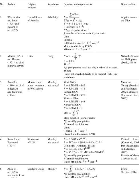
[image:5.612.150.444.67.245.2]Table 2.Summary of different studies that developed rainfall erosivity equations, original locations, and other studies that used their equa-tions.
No. Author Original location
Resolution Equation and requirements Other studies
1 Wischmeier and Smith (1978) and Renard et al. (1997)
United States of America
Sub-daily R=
j P i=1
(EI30)i
N
EI30 =E×I30
E=916+331×log10I I: intensity (in h−1)
EI30i:EI30for stormi
j: number of storms in anN-year period Units
Imperial:
100 foot-ton in acre−1h−1year−1 Metric (multiply by 17.02): MJ mm ha−1h−1year−1
Applied around the USA
2 Mihara (1951) and Hudson (1971) as cited in David (1988)
USA Daily R=A×
n
P 1
Pim A=0.002
M=2
Pi: precipitation total for day i when P exceeds
25 mm
Units: not specified, likely to be original USLE im-perial units
Watersheds around the Philippines (David, 1988)
3 Arnoldus (1980) as cited in Renard and Freimund (1994)
Morocco and other locations in West Africa
Monthly and annual
West Africa:
R=4.79MFI−142
R=5.44MFI−416 Eastern USA:
R=6.86MFI−420 Western USA:
R=4.79MFI−143 Northwest USA:
R=0.66MFI−3 MFI=
12 P
i=1 Pi2
P
MFI: modified Fournier index
Pi: monthly precipitation
P: annual precipitation Units:
t- cm ha−1h−1year−1 (Renard and Freimund, 1994)
Morocco, Turkey (Demirci and Karaburun, 2012); Morocco (Raissouni et al., 2016)
4 Renard and Freimund (1994)
West coast of USA
Monthly and annual
R=0.0483×P1.610
R=587.8−1.219P+0.004105P2
Using MFI (Arnoldus, 1980):
R=0.07397×MFI1.847
R=95.77−6.081MFI+0.4770MFI2
Pi: monthly precipitation
P: annual precipitation Units: MJ mm ha−1h−1year−1
Central America (Kim et al., 2005); Iran (Zakerinejad and Maerker, 2015);
Ecuador (Ochoa-Cueva et al., 2015)
5 Zhou et al. (1995) as cited in Li et al. (2014)
Southern China Monthly R= 12 P
i=1
−1.15527+1.792Pi
Pi: monthly precipitation
Units: MJ mm ha−1h−1year−1
China
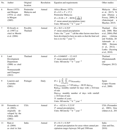
Table 2.Continued.
No. Author Original location
Resolution Equation and requirements Other studies
6 Roose (1975) and Morgan (1974) as cited in Morgan (2005)
Peninsular Malaysia and Africa
Annual Africa (Roose, 1975):
R=0.5×P×17.3 Peninsular Malaysia:
R=(9.28×P−8838)100075 P: mean annual precipitation (mm) Units: MJ mm ha−1h−1year−1
Malaysia (Roslee et al., 2017); Van-uatu (Dumas and Fossey, 2009); Iran (Zakerinejad and Maerker, 2015)
7 El-Swaify et al. (1987) as cited in Merritt et al. (2004)
Possibly Thailand
Annual R=38.5+0.35P
P: mean annual precipitation
Units: t ha−1year−1(all the other factors must have been developed to have no units so that the final soil loss is in t ha−1year−1)
Thailand (Eium-noh, 2000; Merritt et al., 2004); Philip-pines (Adornado and Yoshida, 2010; Adornado et al., 2009; Hernandez et al., 2012); Sri Lanka (Jayasinghe et al., 2010)
8 Land Development Department (2000) as cited in
Nontananandh and Changnoi (2012)
Thailand Annual R=0.04669P−12.1415
P: mean annual rainfall Units: MJ mm ha−1h−1year−1
Thailand (Nontananandh and
Changnoi, 2012)
9 Loureiro and Coutinho (2001)
Portugal Daily R= 1
N N
P
i=1 12 P
m=1
EI30(monthly)
EI30(monthly)=7.05 rain10−88.92 days10 Rain10: monthly rainfall for days with≥10.0 mm of rain
Days10: monthly number of days with rainfall ≥10.0 mm of rain
N: number of years
Units: MJ mm ha−1h−1year−1
Spain
(López-Vicente et al., 2008)
10 Fernandez et al. (2003), originally de-veloped by the USDA-ARS (2002)
USA Annual R= −823.8+5.213P P: annual precipitation Units: MJ mm ha−1h−1year−1
USA (Fernandez et al., 2003); Greece (Jahun et al., 2015)
11 Ram et al. (2004) as cited in Jain and Das (2010)
India Annual R=81.5+0.38P
P: annual precipitation for areas where annual pre-cipitation ranges between 340 and 3500 mm Units: MJ mm ha−1h−1year−1
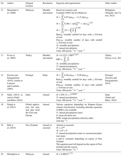
Table 2.Continued.
No. Author Original location
Resolution Equation and requirements Other studies
12 Shamshad et al. (2008)
Malaysia Monthly and annual
Based on Loureiro and
Coutinho (2001) but for Malaysia:
R= 12 P
i=1
6.97 rain10−11.23 days10
R= 12 P
i=1
0.266×rain210.071× days−101.367
R= 12 P
i=1 227×
Pi2 P
0.548
Rain10: monthly rainfall for days with≥10.0 mm of rain
Days10: monthly number of days with rainfall ≥10.0 mm of rain
Pi: monthly precipitation
P: annual precipitation Units: MJ mm ha−1h−1year−1
Philippines (Delgado and Can-ters, 2012)
13 Irvem et al. (2007)
Turkey Monthly and annual
R=0.1215×MFI2.2421 MFI=
12 P
i=1 P2
i P
Pi: monthly precipitation
P: annual precipitation Units: MJ mm ha−1h−1year−1
Turkey
(Ozsoy et al., 2012)
14 Ferreira and Panagopolous (2014), similar to Loureiro and Coutinho (2001)
Portugal Daily R= 12 P
i=1
6.56 rain10−75.09 days10
Rain10: monthly rainfall for days with≥10.0 mm of rain
Days10: monthly number of days with rainfall ≥10.0 mm of rain
Units: MJ mm ha−1h−1year−1
Portugal (Ferreira and Panagopoulos, 2014)
15 Nakil (2014) as cited in Nakil and Khire (2016)
India Annual R=839.15×e0.0008P P: annual precipitation Units: MJ mm ha−1h−1year−1
India (Nakil and Khire, 2016)
18 Naipal et al. (2015)
Global applica-tion, but orig-inal data from the USA and Europe
Annual Various equations depending on Köppen–Geiger climate classification, including alternate equations if SDII is not available
P: annual precipitation (mm) Z: mean elevation (m)
SDII: simple precipitation intensity index (mm day−1)
19 Klik et al. (2015)
New Zealand Annual or seasonal
Annual or seasonal:
R=aPb R=aP+b
P: annual precipitation (mm) or seasonal precipita-tion (mm)
a and b: constants depending on region of New Zealand
The equation used will depend on the region of New Zealand and the season
Units: MJ mm ha−1h−1
20 Sholagberu et al. (2016)
Das (2010) for India. For arid areas, Arnoldus (1980) as cited in Renard and Freimund (1994) has derived erosivity equa-tions for Morocco and other locaequa-tions in West Africa. Many other equations are found in Table 2, and choosing several for sensitivity testing is recommended for future (R)USLE appli-cations. It is also important to test against observed data or Rfactors derived by previous applications in the same study area or in study areas with similar climatic regimes.
2.2 Soil erodibility factor (K)
TheKfactor represents the influence of different soil prop-erties on the slope’s susceptibility to erosion (Renard et al., 1997). It is defined as the “mean annual soil loss per unit of rainfall erosivity for a standard condition of bare soil, re-cently tilled up-and-down slope with no conservation prac-tice” (Morgan, 2005). TheKfactor essentially represents the soil loss that would occur on the (R)USLE unit plot, which is a plot that is 22.1 m long, is 1.83 m wide, and has a slope of 9 % (Lopez-Vicente et al., 2008).
HigherK-factor values indicate the soil’s higher suscepti-bility to soil erosion (Adornado et al., 2009). In the (R)USLE, Wischmeier and Smith (1978) and Renard et al. (1997) use an equation that relates textural information, organic matter, information about the soil structure, and profile permeability with the K factor or soil erodibility factor. However, other soil classifications might not include soil structure and profile permeability information that matches the information re-quired by (R)USLE nomograph. Hence, alternative equations have been developed that exclude the soil structure and pro-file permeability (Table 3). The question of which equation to use depends on the availability of soil data. Where only the textural class and organic matter content are known, Stew-art et al. (1975) have approximatedK-factor values based on these inputs. Similar to theRfactor, the imperial units of soil erodibility are in ton acre hour per hundreds of acres per foot per tonf per inch. Multiplying by 0.1317 gives the erodibility in SI units of metric tons hectare hour per hectare per mega-joule per millimetre (Renard et al., 1997).
Although seemingly relatively straightforward, the K -factor equation proposed by Wischmeier and Smith (1978) comes with a few limitations regarding soil type. This equa-tion was developed using data from medium-textured surface soils in the Midwestern USA, with an upper silt fraction limit of 70 % (Renard et al., 1997). An equation for volcanic soils in Hawaii was proposed by El-Swaify and Dangler (1976) as cited in Renard et al. (1997) but is only appropriate for soils similar to Hawaiian soils and not for all tropical soils. Despite these limitations, many studies outside the USA have used the original Wischmeier and Smith (1978)K-factor equation (Table 3). Being aware of the regional specificity ofK-factor equations is important, and using different K-factor equa-tions in one study area to find a range of soil erodibility could be a way of testing their applicability.
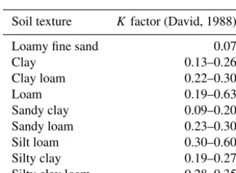
Similar to the sensitivity analysis of the R-factor equa-tions, testing differentK-factor equations to see the variation in erodibility values and then comparing theseKfactors with published values from similar soils would be a good way to test applicability. For the spatial coverage of the European Union, a soil erodibility raster dataset (∼500 m resolution) is available for validation (Panagos et al., 2014). David (1988) and Dymond (2010) have publishedK-factor values for soils of different textural classes (e.g. clay, loam) that can be used if only soil texture is known (Tables 4 and 5). However, the values published by Dymond (2010) are broad and do not account for soils with mixed texture, while the values of David (1988) are based on soils in the Philippines. Like the R factor, it is important to check the derivedK-factor val-ues for the site-specific soil against previously publishedK -factor values for comparable sites and soil types.
2.3 Slope length (L) and steepness (S) factor
TheLSfactor represents the effect of the slope’s length and steepness on sheet, rill, and inter-rill erosion by water, and it is the ratio of expected soil loss from a field slope rela-tive to the original USLE unit plot (Wischmeier and Smith, 1978). The USLE method of calculating the slope length and steepness factor was originally applied at the unit plot and field scale, and the RUSLE extended this to the one-dimensional hill slope scale, with different equations depend-ing on whether the slope had a gradient of more than 9 % (Renard et al., 1997; Wischmeier and Smith, 1978). Further research extends theLSfactor to topographically complex units using a method that incorporates contributing area and flow accumulation (Desmet and Govers, 1996). The USLE and RUSLE method of calculating theLSfactor uses slope length, angle, and a parameter that depends on the steepness of the slope in percent (Wischmeier and Smith, 1978).
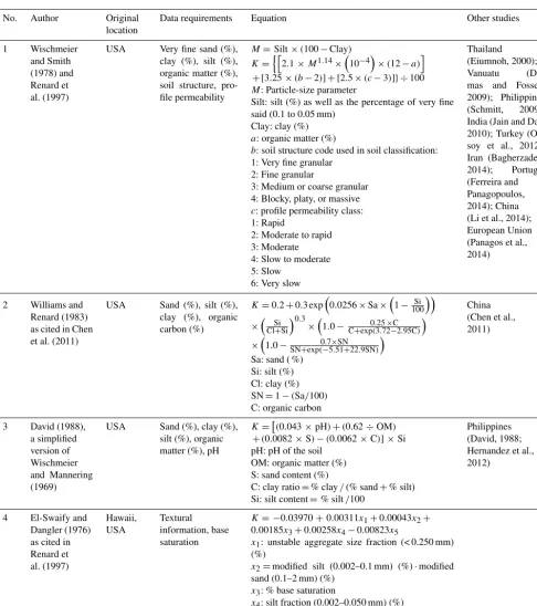
Table 3.Summary of different studies with soil erodibility equations, original locations, and other studies that used their equations. All of the equations in Table 3 use imperial units of soil erodibility: ton acre hour per hundreds of acres per foot per tonf per inch. Multiply by 0.1317 for conversion into SI units of metric ton hours per megajoules per millimetre.
No. Author Original location
Data requirements Equation Other studies
1 Wischmeier and Smith (1978) and Renard et al. (1997)
USA Very fine sand (%), clay (%), silt (%), organic matter (%), soil structure, pro-file permeability
M=Silt×(100−Clay)
K=nh2.1×M1.14×10−4×(12−a)i
+[3.25×(b−2)]+[2.5×(c−3)]} ÷100
M: Particle-size parameter
Silt: silt (%) as well as the percentage of very fine said (0.1 to 0.05 mm)
Clay: clay (%)
a: organic matter (%)
b: soil structure code used in soil classification: 1: Very fine granular
2: Fine granular
3: Medium or coarse granular 4: Blocky, platy, or massive
c: profile permeability class: 1: Rapid
2: Moderate to rapid 3: Moderate 4: Slow to moderate 5: Slow
6: Very slow
Thailand (Eiumnoh, 2000); Vanuatu (Du-mas and Fossey, 2009); Philippines (Schmitt, 2009); India (Jain and Das, 2010); Turkey (Oz-soy et al., 2012); Iran (Bagherzadeh, 2014); Portugal (Ferreira and Panagopoulos, 2014); China (Li et al., 2014); European Union (Panagos et al., 2014)
2 Williams and Renard (1983) as cited in Chen et al. (2011)
USA Sand (%), silt (%), clay (%), organic carbon (%)
K=0.2+0.3 exp0.0256×Sa×1− Si 100
×
Si Cl+Si
0.3 ×
1.0− 0.25×C C+exp(3.72−2.95C)
×
1.0−SN+exp(0−.75×.51SN+22.9SN) Sa: sand ( %)
Si: silt (%) Cl: clay (%) SN=1−(Sa/100)
C: organic carbon
China (Chen et al., 2011)
3 David (1988), a simplified version of Wischmeier and Mannering (1969)
USA Sand (%), clay (%), silt (%), organic matter (%), pH
K=(0.043×pH)+(0.62÷OM)
+(0.0082×S)−(0.0062×C)]×Si pH: pH of the soil
OM: organic matter (%) S: sand content (%)
C: clay ratio=% clay/(% sand+% silt) Si: silt content=% silt/100
Philippines (David, 1988; Hernandez et al., 2012)
4 El-Swaify and Dangler (1976) as cited in Renard et al. (1997)
Hawaii, USA
Textural information, base saturation
K= −0.03970+0.00311x1+0.00043x2+ 0.00185x3+0.00258x4−0.00823x5
x1: unstable aggregate size fraction (< 0.250 mm) (%)
x2=modified silt (0.002–0.1 mm) (%)·modified sand (0.1–2 mm) (%)
x3: % base saturation
x4: silt fraction (0.002–0.050 mm) (%)
Table 4.K-factor values from Dymond (2010) for soil textures in New Zealand.
Soil texture Kfactor (Dymond, 2010)
Clay 0.20
Loam 0.25
Sand 0.05
Silt 0.35
Table 5.K-factor values from David (1988) for soil textures in the Philippines.
Soil texture Kfactor (David, 1988) Loamy fine sand 0.07
Clay 0.13–0.26
Clay loam 0.22–0.30
Loam 0.19–0.63
Sandy clay 0.09–0.20 Sandy loam 0.23–0.30 Silt loam 0.30–0.60 Silty clay 0.19–0.27 Silty clay loam 0.28–0.35
depends on the study area’s scale. The relatively coarse glob-ally available DEMs (∼30 m at best) are less suited to field and sub-catchment scale studies where it may be important to capture effects of micro-topography.
The original equations for the LSfactor assume that slopes have uniform gradients and any irregular slopes would have to be divided into smaller segments of uniform gradi-ents for the equations to be more accurate (Wischmeier and Smith, 1978). At the plot or small field scale, this manual measurement of slopes and dividing into segments may be manageable, but it is less useful at larger scales. In terms of practicality, Desmet and Govers (1996) have reported studies of this method applied at a watershed scale with the disad-vantages of it being time-consuming. Studies in Iran and the Philippines have implemented the (R)USLE methods within a GIS environment by calculating the LSfactor for each raster cell in a DEM, essentially treating each pixel as its own segment of uniform slope (Bagherzadeh, 2014; Schmitt, 2009).
As explained above, the method of using flow accumu-lation, upslope contributing area, and slope in a GIS envi-ronment has gained popularity due to its ability to explicitly account for convergence and divergence of flow, thus captur-ing more complex topography (Wilson and Gallant, 2000). The flow accumulation method was applied at the scales of watersheds and regions (as shown in Table 6) and has even been applied by Panagos et al. (2015a) at the scale of the European Union using a 25 m DEM. The only thing limit-ing users is the availability of high-resolution DEMs and the trade-off between processing time and accuracy. The original
(R)USLE methods require only slope angle and length, op-erate over a single cell in a DEM by treating it as a uniform slope, and take less processing time compared to the method using flow accumulation. However, the user must remember that this cannot capture the convergence and divergence of flow and thus sacrifices accuracy for time.
Additionally, the issue of limited vertical accuracy in global and many national DEMs confounds the uncertain-ties associated with coarse cell sizes. Further work on un-derstanding the appropriate horizontal resolution and verti-cal accuracy of DEMs used for soil erosion predictions at the sub-catchment or field scales is suggested.
Benavidez (2018) investigated use of high-resolution DEMs (15 m and finer), finding the methods that only used slope length and steepness were adequate at delineating large vulnerable areas at the watershed scale. However, the meth-ods using flow accumulation performed significantly better at the sub-watershed or field scale (Benavidez, 2018).
In summary, the choice of whichLS-factor method to use is dependent on the spatial resolution of the DEM, avail-ability of computing resources, and scale of the study site. DEms with spatial resolution coarser than∼100 m do not accurately capture the flow network of a catchment (Pana-gos et al., 2015a). TheLS-factor methods that account for only slope length and steepness are recommended for sites with such coarse DEMs. At the national, regional, or water-shed scale, delineating large areas vulnerable to soil loss is more useful due to the ease of managing these areas at such large scales, and the methods that use only slope length and steepness are recommended. For sub-watershed or field stud-ies and with sufficiently fine DEMs (∼15 m or finer), using LS-factor methods that account for flow accumulation are more useful for identifying the most critical areas of vulner-ability for targeted management approaches.
2.4 Cover and management factor (C)
The cover and management factor (C) is defined as the ratio of soil loss from a field with a particular cover and manage-ment to that of a field under “clean-tilled continuous fallow” (Wischmeier and Smith, 1978). The (R)USLE uses a com-bination of sub-factors such as impacts of previous manage-ment, canopy cover, surface cover and roughness, and soil moisture on potential erosion to produce a value for the soil loss ratio, which is used with theRfactor to produce a value for theCfactor (Renard et al., 1997). This method requires extensive knowledge of the study area’s cover characteristics including agricultural management and may be suitable at the field or farm scale, but monitoring all these characteristics at the watershed scale may not be feasible.
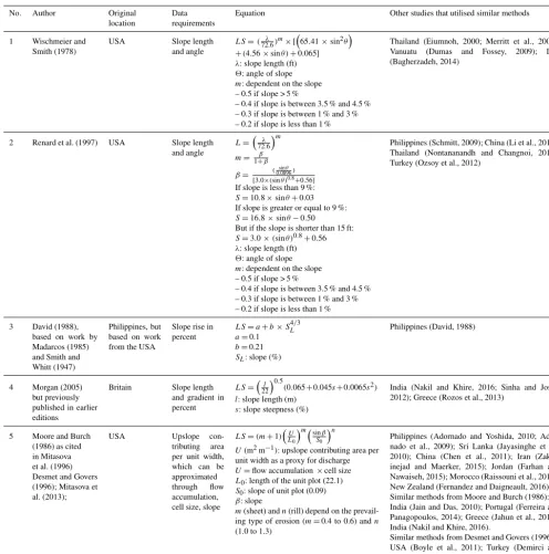
[image:11.612.84.251.213.335.2]in-Table 6.Summary of methods of calculatingLSfactor, original locations, and other studies that used these methods.
No. Author Original
location
Data requirements
Equation Other studies that utilised similar methods
1 Wischmeier and Smith (1978)
USA Slope length
and angle
LS=(72λ.6)m× [65.41×sin2θ
+(4.56×sinθ )+0.065]
λ: slope length (ft)
2: angle of slope
m: dependent on the slope – 0.5 if slope > 5 %
– 0.4 if slope is between 3.5 % and 4.5 % – 0.3 if slope is between 1 % and 3 % – 0.2 if slope is less than 1 %
Thailand (Eiumnoh, 2000; Merritt et al., 2004); Vanuatu (Dumas and Fossey, 2009); Iran (Bagherzadeh, 2014)
2 Renard et al. (1997) USA Slope length and angle
L=
λ
72.6
m
m= β
1+β
β= (
sinθ
0.0896)
[3.0×(sinθ )0.8+0.56] If slope is less than 9 %:
S=10.8×sinθ+0.03 If slope is greater or equal to 9 %:
S=16.8×sinθ−0.50
But if the slope is shorter than 15 ft:
S=3.0×(sinθ )0.8+0.56
λ: slope length (ft)
2: angle of slope
m: dependent on the slope – 0.5 if slope > 5 %
– 0.4 if slope is between 3.5 % and 4.5 % – 0.3 if slope is between 1 % and 3 % – 0.2 if slope is less than 1 %
Philippines (Schmitt, 2009); China (Li et al., 2014); Thailand (Nontananandh and Changnoi, 2012); Turkey (Ozsoy et al., 2012)
3 David (1988), based on work by Madarcos (1985) and Smith and Whitt (1947)
Philippines, but based on work from the USA
Slope rise in percent
LS=a+b×SL4/3 a=0.1
b=0.21
SL: slope (%)
Philippines (David, 1988)
4 Morgan (2005) but previously published in earlier editions
Britain Slope length and gradient in percent
LS=l
22
0.5
(0.065+0.045s+0.0065s2)
l: slope length (m)
s: slope steepness (%)
India (Nakil and Khire, 2016; Sinha and Joshi, 2012); Greece (Rozos et al., 2013)
5 Moore and Burch (1986) as cited in Mitasova et al. (1996) Desmet and Govers (1996); Mitasova et al. (2013);
USA Upslope
con-tributing area per unit width, which can be approximated through flow accumulation, cell size, slope
LS=(m+1)U
L0 msinβ
S0 n
U(m2m−1): upslope contributing area per unit width as a proxy for discharge
U=flow accumulation×cell size
L0: length of the unit plot (22.1) S0: slope of unit plot (0.09) β: slope
m(sheet) andn(rill) depend on the prevail-ing type of erosion (m=0.4 to 0.6) andn
(1.0 to 1.3)
Philippines (Adornado and Yoshida, 2010; Ador-nado et al., 2009); Sri Lanka (Jayasinghe et al., 2010); China (Chen et al., 2011); Iran (Zaker-inejad and Maerker, 2015); Jordan (Farhan and Nawaiseh, 2015); Morocco (Raissouni et al., 2016); New Zealand (Fernandez and Daigneault, 2016). Similar methods from Moore and Burch (1986): India (Jain and Das, 2010); Portugal (Ferreira and Panagopoulos, 2014); Greece (Jahun et al., 2015); India (Nakil and Khire, 2016).
Similar methods from Desmet and Govers (1996): USA (Boyle et al., 2011); Turkey (Demirci and Karaburun, 2012); Philippines (Delgado and Can-ters, 2012).
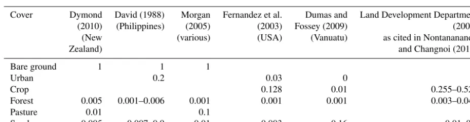
clude the effect of percent ground cover, reportingC-factor values for the same cover type over a range of cover percent-age and condition. Morgan (2005) and David (1988) have reported values for the different growth stages of the same types of trees. A simple method of creating aC-factor layer is by using lookup tables to assignC-factor values to the land cover classes present in the study area. When usingCfactors from the literature, it is important to note that the definition of land cover type between two countries may vary. For
[image:12.612.48.544.83.583.2]Table 7.C-factor equations that use NDVI.
No. Author Original location Equation
1 Van der Knijff et al. (2000)
Europe C=exp h
∝
NDVI β−NDVI
i
α=2
β=1 2 Ma et
al. (2010) as cited in Li et al. (2014)
China fg= NDVINDVImax−−NDVINDVIminmin
C=
1 fg=0
0.6508−0.343×log?(fg) 0< fg<78.3%
0 fg≥78.3%
Table 8.Cfactors for general types of land cover compiled from various sources.
Cover Dymond David (1988) Morgan Fernandez et al. Dumas and Land Development Department (2010) (Philippines) (2005) (2003) Fossey (2009) (2002) (New (various) (USA) (Vanuatu) as cited in Nontananandh
Zealand) and Changnoi (2012)
Bare ground 1 1 1
Urban 0.2 0.03 0 0
Crop 0.128 0.01 0.255–0.525
Forest 0.005 0.001–0.006 0.001 0.001 0.001 0.003–0.048
Pasture 0.01 0.1
Scrub 0.005 0.007–0.9 0.01 0.003 0.16 0.01–0.1
reason why using the lookup-table-based approach is inade-quate and tedious.
To address this, another method of determining the Cfactor is through the normalized difference vegetation in-dex (NDVI) estimated from satellite imagery. Although there are NDVI layers available, these are limited by geographical coverage, date of acquisition, and resolution. The MODIS NDVI dataset made by Caroll et al. (2004) at 250 m resolu-tion covers the USA and South America2. NASA produced a global dataset of NDVI values at 1◦resolution for the time span of July 1983 to June 1984, making it suitable for study-ing historical soil erosion but not necessarily for the current state of land cover3.
In areas where ready-made NDVI products are unavail-able, authors have used satellite imagery to obtain NDVI such as AVHRR or Landsat ETM (Van der Knijff et al., 2000; De Asis and Omosa, 2007; Ma et al., 2010, as cited in Li et al., 2014). De Asis and Omasa (2007) related the Cfactor and NDVI through fieldwork and image classification – de-termining theCfactor at several points within the study area using the (R)USLE approach and relating it to the NDVI through regression correlation analysis. This may not be fea-sible in larger study areas such as the European Union, where Van der Knijff et al. (2000) determined NDVI from
satel-2http://glcf.umd.edu/data/ndvi/ (last access: 12 November 2018)
3https://data.giss.nasa.gov/landuse/ndvi.html (last access:
12 November 2018)
lite imagery and created an equation based on its positive correlation with green vegetation (Table 7). This approach enabled them to create aC-factor map over the European Union. However,Cfactors were unrealistically high in some areas such as woodland and grassland, so values for those areas were taken from the literature.
An advantage of using NDVI is that researchers can deter-mine sub-annualCfactors if there is satellite imagery avail-able, which can lead to understanding the contribution of cover to seasonal soil erosion and identifying critical peri-ods within the year where soil erosion is a risk (Ferreira and Panagopoulos, 2014). Similar methods have been applied in Brazil by Durigon et al. (2014), Greece by Alexandridis et al. (2015), and Kyrgyzstan by Kulikov et al. (2016). Deter-miningC factors at the seasonal scale is important because vegetation cover can change throughout the year due to agri-cultural and forestry practices. In study areas with a high temporal variation of rainfall throughout the year, seasonal vegetation can play a big part in exacerbating or mitigating soil erosion.
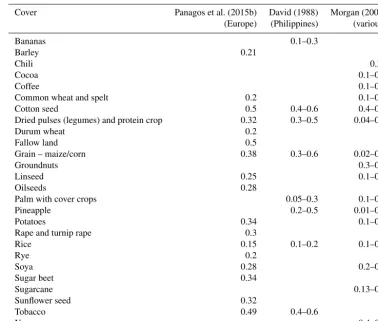
[image:13.612.65.529.237.358.2]Table 9.Cfactors for specific types of land cover compiled from various sources.
Cover Panagos et al. (2015b) David (1988) Morgan (2005) (Europe) (Philippines) (various)
Bananas 0.1–0.3
Barley 0.21
Chili 0.33
Cocoa 0.1–0.3
Coffee 0.1–0.3
Common wheat and spelt 0.2 0.1–0.4
Cotton seed 0.5 0.4–0.6 0.4–0.7
Dried pulses (legumes) and protein crop 0.32 0.3–0.5 0.04–0.7
Durum wheat 0.2
Fallow land 0.5
Grain – maize/corn 0.38 0.3–0.6 0.02–0.9
Groundnuts 0.3–0.8
Linseed 0.25 0.1–0.2
Oilseeds 0.28
Palm with cover crops 0.05–0.3 0.1–0.3
Pineapple 0.2–0.5 0.01–0.4
Potatoes 0.34 0.1–0.4
Rape and turnip rape 0.3
Rice 0.15 0.1–0.2 0.1–0.2
Rye 0.2
Soya 0.28 0.2–0.5
Sugar beet 0.34
Sugarcane 0.13–0.4
Sunflower seed 0.32
Tobacco 0.49 0.4–0.6
Yams 0.4–0.5
Table 10.Examples of whereCfactor accounts for crop management from Morgan (2005) and David (1988).
Crop Management Cfactor
Maize, sorghum, or millet High productivity; conventional tillage 0.20–0.55 Low productivity; conventional tillage 0.50–0.90 High productivity; chisel ploughing into residue 0.12–0.20 Low productivity; chisel ploughing into residue 0.30–0.45 High productivity; no or minimum tillage 0.02–0.10
Coconuts Tree intercrops 0.05–0.1 Annual crops as intercrop 0.1–0.30
NDVI. At small scales and with a good understanding of dif-ferences in land cover classifications, pulling values from the literature may be the most efficient choice, but at larger re-gional scales this may become tedious. At larger scales, high-resolution satellite imagery may be available to determine NDVI, but authors must be mindful of its acquisition date in relation to their study period, as well as data quality and im-age processing issues such as dealing with cloud cover and aggregating images from multiple satellite passes (Van der Knijff et al., 2000; Kulikov et al., 2016).
2.5 Support practice factor (P)
[image:14.612.129.466.441.548.2]sup-port practices observed, theP factor is 1.0 (Adornado et al., 2009). TheP factor can also be estimated using sub-factors, but the difficulty of accurately mapping support practice fac-tors or not observing support practices leads to many studies ignoring it by giving theirP factor a value of 1.0 as seen in Appendix A1 (Adornado et al., 2009; Renard et al., 1997; Schmitt, 2009).
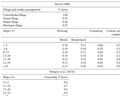
Another possible reason why studies may ignore the P factor is due to the nature of their chosenCfactors. Some C factors already account for the presence of a support fac-tor such as intercropping or contouring. For example, Mor-gan (2005) and David (1988) give C factors for one type of crop, but with different types of management (Table 10). Despite theP factor being commonly ignored, a number of studies have reported possibleP factors for different kinds of tillage, terracing, contouring, and strip cropping (Table 11). TheP factor has a significant impact on the estimation of soil loss. For example, aP factor of 0.25 for zoned tillage reflects the potential for this management factor to reduce soil by 75 % loss compared to conventional tillage (P factor: 1.00). At suitably detailed scales and with enough knowledge of farming practices, using theseP factors may lead to a more accurate estimation of soil loss. Additionally, theseP factors can be used in scenario analysis to understand how chang-ing farmchang-ing practices may mitigate or exacerbate soil loss. An application of (R)USLE in the Cagayan de Oro catch-ment in the Philippines showed, through scenario analysis, that soil conservation practices such as agroforestry and al-ley cropping could potentially lead to large decreases in soil loss compared to the baseline scenario (Benavidez, 2018).
In summary, including theP factor in (R)USLE applica-tions is important because of the significant effects that some management practices can have on reducing soil loss com-pared to conventional tillage. TheP factor is useful for stud-ies where different management practices are being consid-ered for the same site as it can elucidate which practices are more beneficial for soil conservation.
3 Limitations of (R)USLE
This section presents a few of the key limitations of the (R)USLE: regional applicability, uncertainties associated with the model, input data and validation, and representing other types of erosion.
The most commonly cited limitation of the (R)USLE mod-els is their reduced applicability to regions outside of the United States of America (Aksoy and Kavvas, 2005; Naipal et al., 2015; Sadeghi et al., 2014). The original USLE was formulated based on soil erosion studies on agricultural land in the USA. When applied to different climate regimes and land cover conditions, this may lead to greater uncertain-ties associated with estimates of average annual soil loss (Kinnell, 2010). Since the (R)USLE parameters were devel-oped based on small-scale studies of agricultural plots, there
are also uncertainties associated with upscaling the original USLE to the catchment or regional scale (Nagle et al., 1999; Naipal et al., 2015). Wischmeier and Smith (1987) have also warned that using the (R)USLE in conditions extremely dif-ferent from the agricultural conditions the model was formu-lated under may lead to extrapolation error. Of the studies reviewed for this paper (Table A1), most applications were done on catchments with predominantly agricultural land use, but under a range of different climatic conditions.
Sensitivity analysis and testing which (R)USLE sub-factors suit particular study sites is one method of addressing the (R)USLE’s regional applicability. Like the Mangatarere application method in Sect. 2.1, other studies have tested multipleR-factor equations on the same dataset to determine which equation was most appropriate for their study site (Eiumnoh, 2000; Benavidez, 2018). Their derivedR-factor values were compared to the values for catchments with sim-ilar climate and rainfall, or to maps of theRfactor at larger spatial scales (Panagos et al., 2017). To reduce uncertainty in accounting for land use, work by Post and Hartcher (2005) recommended usingC-factor values for specific land cover classifications (e.g. specific crops, forest growth stages) in-stead of values for broad land cover categories (e.g. agricul-ture, forest). AlthoughC-factor values can be taken from the literature or determined in situ, an extensive literature review compiling potential soil loss rates of different crop and for-est covers compared to likely soil loss rates of bare soil can be used to determine likelyC-factor values of a particular site. Improvements and modifications to the (R)USLE sub-factors have made it applicable to larger spatial scales, in-cluding a coarse-resolution representation at the global scale (Naipal et al., 2015). The pan-European application by Pana-gos et al. (2015a) showed setting a maximum value for slope steepness of 50 % (26.6◦) would prevent significantly large LS-factor values and account for the absence of soil on such steep slopes. Assembling published estimates of (R)USLE sub-factors from different climatic regions and soil types would help in sensitivity testing (R)USLE equations, decid-ing the most appropriate equation to use, and verifydecid-ing the derived (R)USLE sub-factor values.
The uncertainties associated with the (R)USLE, and ar-guably soil erosion modelling in general, stem from several factors: the inability of models to capture the complex in-teractions involved in soil loss, the low availability of long-term reliable data for modelling, and the lack of soil erosion observational data for model validation, especially in data-scarce environments. The simplicity of the (R)USLE allows usage in locations where there are insufficient data for more complex models that require large input datasets (de Vente and Poesen, 2005; Hernandez et al., 2012). Of the studies reviewed, very few critically discuss the uncertainties asso-ciated with the (R)USLE, but those that do offer several ways to overcome these uncertainties.
Table 11.P factors for different types of agricultural management practices.
David (1988)
Tillage and residue management P factor Conventional tillage 1.00
Zoned tillage 0.25
Mulch tillage 0.26
Minimum tillage 0.52
Slope (%) Terracing Contouring Contour strip cropping
Bench Broad-based
1–2 0.10 0.12 0.60 0.30
3–8 0.10 0.10 0.50 0.15
9–12 0.10 0.12 0.60 0.30
13–16 0.10 0.14 0.70 0.35
17–20 0.12 0.16 0.80 0.40
21–25 0.12 0.18 0.90 0.45
> 25 0.14 0.20 0.95 0.50
Panagos et al. (2015c)
Slope (%) ContouringP factor
9–12 0.6
13–16 0.7
17–20 0.8
21–25 0.9
> 25 0.95
erosion rates should be taken as best estimates rather than ab-solute values (Wischmeier and Smith, 1987). Some applica-tions have chosen to display their soil loss results as categor-ical to produce maps that show low, medium, or high areas of vulnerability instead of showing annual average amounts (Adornado et al., 2009; Schmitt, 2009). The (R)USLE is a good first attempt at identifying vulnerable areas and esti-mating soil loss for a landscape at the baseline scenario due to the model’s relative simplicity and few data requirements (Aksoy and Kavvas, 2005). The (R)USLE is also useful for doing scenario analysis to check whether changing land use or management practices would either exacerbate or mitigate soil loss, making it useful for comparison purposes (Merritt et al., 2004; Nigel and Rughooputh, 2012).
Validating the soil erosion rates produced by the (R)USLE is difficult because of the lack of easily obtainable obser-vational soil erosion records, especially in data-scarce en-vironments. Out of the (R)USLE applications reviewed for this paper, ∼30 % presented explicit comparisons between their modelled soil loss from (R)USLE and observed soil loss, modelled soil loss from (R)USLE and other models (one study), and soil loss from multiple models and observed soil loss (one study).
One study compared the soil loss rates predicted by the RUSLE to estimates of the physically based WEPP (Water
Erosion Prediction Project) model. Amore et al. (2004) com-pared RUSLE and WEPP and found that the ratio of mod-elled to observed soil loss of WEPP (0.7) was better than RUSLE (0.2) for the Trinità basin. However, both RUSLE and WEPP over-predicted sediment yield by up to 5 times the observed value for the nearby Ragoleto basin (Amore et al., 2004). Although WEPP also estimates rill and inter-rill erosion, WEPP is a continuous daily model that accounts for deposition and sediment delivery, which RUSLE does not predict (Aksoy and Kavvas, 2005).
Another study compared the soil loss estimates of the RUSLE and Unit Stream Power Erosion Deposition Model (USPED) to each other, and to observed data. In a compari-son between the RUSLE and USPED, the ratio of modelled to observed of soil loss was almost unity for the USPED but 0.86 for the RUSLE (Aiello et al., 2014). The USPED model builds and improves on the RUSLE sub-factors through its ability to incorporate overland flow and sediment transport through the landscape (Aiello et al., 2014; Zakerinejad and Maerker, 2015).
under-predicted soil loss cited the model’s inability to ac-count for gully erosion and mass wasting as one of the rea-sons for estimation errors, thus underscoring the importance of including these types of erosion in future improvements to RUSLE (Dabney et al., 2012; Gaubi et al., 2017). An-other issue is differences in temporal and/or spatial resolu-tion and sometimes differing timescales between modelled and observed estimates. Average observations based on oc-casional grab samples of sediment in streams may not well represent the monthly to annual sediment loads the (R)USLE is attempting to estimate. In another example, López-Vicente et al. (2008) compared observed to modelled values and had a ratio of modelled to observed soil loss of 0.62. However, the “observed” soil loss was based on 137Cs measurements that were indicative of average soil loss values for the past 40 years, while the model values were based on 1997–2006 driving data. During this period, the study area experienced lower precipitation and thus had lower modelled soil loss measurements compared to the soil loss derived from the
137Cs records (López-Vicente et al., 2008).
As stated earlier, the regional applicability of the RUSLE is a limitation that requires the sub-factors to be adjusted and modified based on the specific characteristics of the re-searcher’s study site. Nakil and Khire (2016) and Abu Ham-mad et al. (2005) show this important practice in RUSLE ap-plications in their studies. Through testing and refining their method of accounting for topography through theLSfactor, the ratio of modelled to observed soil loss ranged from 0.8 to almost unity (Nakil and Khire, 2016). The initial applica-tion of RUSLE of Abu Hammad et al. (2005) over-estimated soil loss by a factor of 3, but with adjustments to the sub-factors based on local data on soil moisture, land cover, and support practices, the model error was reduced to 14 %. The importance of adjusting RUSLE with the availability of more detailed data was further shown in the pan-European study of Panagos et al. (2015e), where detailed soil, topography, land cover, and management practices allowed the researchers to refine their application where most of the ratios of modelled to observed soil loss were very good (0.9 to 1.3). In the validation areas where the soil loss comparisons were not good, further local testing and refining of the RUSLE sub-factors is seen as an area in which to improve the model re-sults (Beskow et al., 2009; Ozsoy et al., 2012; Panagos et al., 2015e).
A global soil erosion study using RUSLE was accom-plished by Borrelli et al. (2017) using the rainfall erosivity map generated by Panagos et al. (2017) that showed com-parable results to regional and local soil erosion estimates, and good agreement with global soil erosion datasets such as the Global Assessment of Human-induced Soil Degradation (GLASOD) dataset4.
4https://www.isric.online/projects/
global-assessment-human-induced-soil-degradation-glasod (last access: 12 November 2018)
Future work in the soil erosion literature could include assembling a comprehensive database of global, regional, and national soil erosion rates to allow comparison between soil erosion modelling methods, not just (R)USLE results. A proxy for understanding soil erosion is water quality data such as total suspended solids (TSS) that includes sediment delivery and organic sources (Schmitt, 2009; Russo, 2015). However, TSS usually excludes the larger and heavier bed-load sediments that could be resulting from mass wasting events or erosion (Nagle et al., 1999). Nevertheless, water quality data are useful for inferring likely temporal patterns of soil erosion or the sediment yield during seasons of heavy rainfall or after extreme events. Ground truthing or analysis of satellite imagery is another useful method of validating the (R)USLE results, as the areas of extreme erosion risk can be checked for physical evidence of soil loss occurrence (De Asis and Omasa, 2007; Adornado and Yoshida, 2010; Non-tananandh and Changnoi, 2012). The soil loss estimates can be validated against observations from similar catchments, recorded events of mass wasting, or larger-scale soil loss studies at the national or regional scale (Životi´c et al., 2012; Panagos et al., 2015e; Nakil and Khire, 2016).
Lastly, a frequently cited limitation is that the (R)USLE es-timates soil loss through sheet and rill erosion, but not from other types of erosion such as gully erosion, channel erosion, bank erosion, or mass wasting events such as landslides (Na-gle et al., 1999; Wischmeier and Smith, 1978). By excluding these types of erosion, the (R)USLE may underestimate the actual soil loss (Thorne et al., 1985). The model also does not account for deposition, leading to overestimation, or sed-iment routing (Desmet and Govers, 1996; Wischmeier and Smith, 1978). Since it does not predict the sediment path-ways from hill slopes to water bodies, it is difficult to analyse possible effects on downstream areas, such as pollution or sedimentation (Jahun et al., 2015). One of the possible meth-ods for linking the (R)USLE results to sediment delivery to streams is using the sediment delivery ratio (SDR), defined as “the ratio of the sediment delivered at a location in the stream system to the gross erosion from the drainage area above that point” (Yoon et al., 2009). This parameter varies depending on the gradient, slope shape, and length and can also be influenced by land cover, roughness, etc. (Wu et al., 2005). Given that it is influenced by characteristics similar to those of the (R)USLE, future work can include not only com-bining the (R)USLE with the SDR to estimate sediment de-livery to streams but also avoiding possible double counting. These two limitations of deposition and routing are linked to the model’s representation of more topographically complex terrain, and previous studies have attempted to address them by improving on the LSfactor by incorporating upstream contributing area (Desmet and Govers, 1996; Moore et al., 1991). A more detailed discussion of addressing these limi-tations is in Sect. 4.1.
data requirements compared to more complex physically based models. Studies around the world continue to improve (R)USLE parameterisation and application in different cli-mate regimes and locations.
4 Future directions
Since the (R)USLE and its family of models are used over different geographic locations and climate types, it is impor-tant for future research to build on them and improve their representation of real-world soil loss. Some of the future di-rections include incorporating soil loss from other types of erosion, estimating soil loss at seasonal or sub-annual tem-poral scales, and improving the consistency of formulae and units in the scientific literature.
4.1 Representing other types of erosion
As previously discussed in Sect. 3, the (R)USLE does not account for all erosion types. This section mostly discusses possible extensions to include gully erosion, but further work to incorporate channel/bank erosion and mass wasting events must also be done.
The inability of (R)USLE to account for soil losses due to ephemeral gullies can lead to under-prediction of soil loss estimates (Thorne et al., 1985). These ephemeral gullies are small channels that form due to the erosive action of over-land flow during a rainfall event (Momm et al., 2012). Gully erosion can contribute a significant amount of sediment loss; for example gully erosion is estimated to contribute between 30 % and 50 % of soil loss from a range of catchments in New Zealand (Basher et al., 2012). Desmet and Govers (1996) recommended that delineation of ephemeral gullies, such as through the Compound Topographic Index (CTI) developed by Thorne et al. (1985), combined with (R)USLE could im-prove the identification of vulnerable areas within a water-shed. The CTI of Thorne et al. (1985) uses topographic anal-ysis to predict locations and soil loss rates of ephemeral gul-lies based on upstream drainage area, slope, and the planform curvature. Hence, the combination of CTI and the (R)USLE is a promising direction for including gully erosion, but care must be taken in coupling these models because both already account for upstream drainage area and slope. Simply adding their soil loss rates could lead to “double counting” and re-quires further research to determine the threshold values of CTI andLSfactor over which ephemeral gullying is likely (Benavidez, 2018).
Work along these lines, combining the effect of rill and sheet erosion with gully erosion was done by Momm et al. (2012) in Kansas and by Zakerinejad and Maeker (2015) in the Mazayjan watershed in Iran. Momm et al. (2012) com-bined several types of erosion – sheet and rill, gully, and bed and bank erosion – with the sheet and rill erosion es-timated using the (R)USLE model. They used varying
criti-cal CTI thresholds to iteratively generate potential locations of ephemeral gullies and identify sub-watersheds prone to gully erosion, and then used scenario analysis to estimate reductions in sediment yields under conservation practices (Momm et al., 2012). One of the limitations of the Momm et al. (2012) study was that they only had a coarse-resolution DEM. Since ephemeral gullies are small features (typically a few metres wide and ∼25 cm deep), higher-resolution DEMs such as those derived from lidar data would be bet-ter for analysis of these topographic features. The USPED, which is similar to the (R)USLE model, has also been used to estimate rill and sheet erosion rates with a stream power index (SPI) approach to estimate gully erosion rates (Zaker-inejad and Maerker, 2015). Zaker(Zaker-inejad and Maerker (2015) estimated gully erosion in metric tons per hectare per year and combined it with the estimates from the USPED model to produce a map showing potential erosion and deposition within their study area. Hence, there are precedents as well as a need to combine erosion estimates from (R)USLE with a procedure that accounts for gully erosion for more effective land management.
4.2 Seasonal erosion vulnerability
(R)USLE applications usually estimate soil loss at the an-nual timescale, and the MUSLE estimates soil loss from a single storm event (Renard et al., 1997; Sadeghi et al., 2014). As seen in the review of methods of calculating rain-fall erosivity, many different studies have attempted to esti-mate theR factor, underscoring its importance to soil ero-sion research. However, estimating theRfactor at the annual timescale does not account for seasonal variations in rainfall. It is useful for land management to understand seasonal vari-ations in soil erosion vulnerability because of the dual effect of rainfall and land cover on soil loss, and the effect of rain-fall on land cover (Kulikov et al., 2016). For example, when a season of heavy rainfall coincides with low vegetation cover, the risk of soil erosion increases considerably (Ferreira and Panagopoulos, 2014). Thus, most of the studies around sea-sonal estimations of soil loss revolve around changes in land cover and rainfall. The soil erodibility (K factor) can vary too due to changes in permeability and the effects of freez-ing and thawfreez-ing, but it is less frequently studied compared to variations in land cover and rainfall (López-Vicente et al., 2008).