www.hydrol-earth-syst-sci.net/16/1419/2012/ doi:10.5194/hess-16-1419-2012
© Author(s) 2012. CC Attribution 3.0 License.
Earth System
Sciences
Evaluation of water-energy balance frameworks to predict the
sensitivity of streamflow to climate change
M. Renner1, R. Seppelt2, and C. Bernhofer1
1Technische Universit¨at Dresden, Faculty of Forest-, Geo- and Hydro Sciences – Institute of Hydrology and Meteorology – Chair of Meteorology, Pienner Str. 23, 01737 Tharandt, Germany
2Helmholtz Centre for Environmental Research – UFZ, Department of Computational Landscape Ecology, Permoserstr. 15, 04318 Leipzig, Germany
Correspondence to: M. Renner ([email protected])
Received: 15 September 2011 – Published in Hydrol. Earth Syst. Sci. Discuss.: 27 September 2011 Revised: 10 April 2012 – Accepted: 3 May 2012 – Published: 15 May 2012
Abstract. Long term average change in streamflow is a ma-jor concern in hydrology and water resources management. Some simple analytical methods exist for the assessment of the sensitivity of streamflow to climatic variations. These are based on the Budyko hypothesis, which assumes that long term average streamflow can be predicted by climate con-ditions, namely by annual average precipitation and evapora-tive demand. Recently, Tomer and Schilling (2009) presented an ecohydrological concept to distinguish between effects of climate change and basin characteristics change on stream-flow. We relate the concept to a coupled consideration of the water and energy balance. We show that the concept is equiv-alent to the assumption that the sum of the ratio of annual actual evapotranspiration to precipitation and the ratio of ac-tual to potential evapotranspiration is constant, even when climate conditions are changing.
Here, we use this assumption to derive analytical solu-tions to the problem of streamflow sensitivity to climate. We show how, according to this assumption, climate sensitivity would be influenced by different climatic conditions and the actual hydrological response of a basin. Finally, the proper-ties and implications of the method are compared with estab-lished Budyko sensitivity methods and illustrated by three case studies. It appears that the largest differences between both approaches occur under limiting conditions. Specifi-cally, the sensitivity framework based on the ecohydrologi-cal concept does not adhere to the water and energy limits, while the Budyko approach accounts for limiting conditions by increasing the sensitivity of streamflow to a catchment pa-rameter encoding basin characteristics. Our findings do not
support any application of the ecohydrological concept un-der conditions close to the water or energy limits, instead we suggest a correction based on the Budyko framework.
1 Introduction
In this paper we consider the question how variations in cli-mate affect the hydrological response of river basins. Thus, we aim to assess climate sensitivity of basin streamflow
Qand evapotranspiration ET, (Dooge, 1992; Arora, 2002;
Yang and Yang, 2011; Roderick and Farquhar, 2011). To do so, we need to consider the concurrent climate itself, because naturally the supply of water and energy is the main control-ling factor of evapotranspiration (Budyko, 1974; Zhang et al., 2004; Teuling et al., 2009). Basin characteristics are also of high relevance: two basins with similar climate may have quite different hydrological responses (Yang et al., 2008). Spatio-temporal patterns of precipitation, soils, topography, vegetation and not least human activities have considerable impacts (Arnell, 2002; Milly, 1994; Gerrits et al., 2009; Zhang et al., 2001; Donohue et al., 2007).
Usually, one is tempted to represent such basin character-istics by conceptual or physically based hydrological mod-els. However, the uncertainties arising from model structure and calibration may lead to biased and parameter depen-dent climate sensitivity estimates (Nash and Gleick, 1991; Sankarasubramanian et al., 2001; Zheng et al., 2009).
effects from land-use change effects on streamflow. They uti-lize two non-dimensional ecohydrologic state variables rep-resenting water and energy balance components, which de-scribe the hydro-climatic state of a basin and carry infor-mation of how water and energy fluxes are partitioned at the catchment scale. The central hypothesis of Tomer and Schilling (2009) is that from the observed shift of these states, the type of change can be deduced. Their theory is based on experiments with different agricultural conservation treatments of four small field size experimental watersheds (30–61 ha). They observed that watersheds with different soil conservation treatments also showed different evapotran-spiration ratios. Further, the shift within this hydro-climatic state space due to conservation treatments was perpendicular to the shift which was observed over time. They attributed this temporal shift to a climatic change characterised by in-creased annual precipitation.
The conceptual model proposed by Tomer and Schilling (2009) has great scientific appeal, because of its potential to easily separate climatic from land use effects on the water balance. Here, we aim to explore this potential of the frame-work to address the following research questions:
1. Can this concept also be used to predict stream-flow/evapotranspiration change based on a climate change signal?
2. What are the implications of such a model, given the range of possible hydro-climatic states and changes therein?
3. How does it compare to existing climate sensitivity approaches?
This paper is structured as follows. In the methodologi-cal section we embed the conceptual model of Tomer and Schilling (2009) into a coupled water and energy balance framework. With that we derive analytical solutions, which can be used to predict the sensitivity of streamflow to climate changes.
We then discuss the properties and implications of the new method. We compare our results with previous studies, namely those which employed the Budyko hypothesis for the assessment of streamflow sensitivity (Dooge, 1992; Arora, 2002; Roderick and Farquhar, 2011). In a second paper (Ren-ner and Bernhofer, 2011), we will address the application of this hydro-climatic framework on a multitude of catchments throughout the contiguous United States.
2 Theory
In this section we aim to derive a general framework for the analysis and estimation of long term average changes in basin evapotranspiration and streamflow. The theory is based on the water and energy balance equations, valid for an area such as a watershed or river basin. We revisit the
conceptual framework by Tomer and Schilling (2009) and employ it to derive analytical solutions for (a) the sensitiv-ity of a given basin to climate changes and (b) the expected changes in basin evapotranspiration and streamflow under a given change in climate.
2.1 Coupled water and energy balance
Actual evapotranspirationET links the catchment water and
energy balance equations:
P =ET +Q+1Sw and (1)
Rn=ETL+H+1Se. (2)
The water balance equation expresses the partitioning of pre-cipitation P into the water fluxes ET, streamflow Q
(ex-pressed as an areal estimate) and1Swwhich is the change in water storage. The energy balance equation describes, how available energy, expressed as net radiationRn, is divided at the earth surface into the turbulent fluxes, latent heat flux
ETL, whereLdenotes the latent heat of vaporization, the
sensible heat fluxH and the change in energy storage1Se. As we regard the temporal scale of long term averages and thus consider the integral effect of a range of possible pro-cesses involved, we can assume that both, the change in water and in energy storage, are zero. Dividing the energy balance equation by the latent heat of vaporizationL, both balance equations have the unit of water fluxes, usually expressed as mm per time. Further, the termRn/L, can also be denoted as potential evapotranspirationEp, and expresses the typical upper limit of potential evapotranspiration (Budyko, 1974; Arora, 2002). With the above simplification we can write the energy balance equation as:
Ep=ET +H /L. (3)
2.2 The ecohydrologic framework for change attribution
In the long term, actual basin evapotranspiration ET is
mainly limited by water supply P and energy supply Ep, which considered together, determine a hydro-climatic state space (P,Ep,ET).
Regarding long term average changes in the hydrological states, these must be caused either by a change in climatic conditions, by changes in basin conditions or a combination of both, quietly assuming that our data is homogeneous over time. The conceptual model of Tomer and Schilling (2009) aims to distinguish between both types of causes. They em-ploy two non-dimensional variables, relative excess energy
U and relative excess waterW, which can be obtained by normalizing, both the water balance and the energy balance byP andEp, respectively:
W =1−ET
P =
Q
P, U =1− ET
Ep
= H /L Ep
So, relative excess water W describes the proportion of available water not used by the ecosystem, which is in the case of a catchment the runoff ratioQ/P. Similarly, the re-maining proportion of the available energy not used for evap-otranspiration is expressed as relative excess energyU. Usu-ally both terms are within the interval (0, 1], becauseET is
generally positive, it cannot be larger thanP and it is mostly smaller thanEp(excluding cases with a negative Bowen
ra-tio). These limits are also known as the water and energy lim-its proposed by Budyko (1974). The relation of both terms is essentially a coupled consideration of water and energy bal-ances, to which we will refer to as theU Wspace. So plotting
UversusW in a diagram depicts the relative partitioning of water and energy fluxes of a given basin.
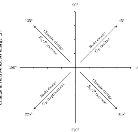
The long term average state expressed byWandUcan be thought of as a steady state balancing water and energy fluxes through coupling between soil, vegetation, hydromorphol-ogy and atmosphere (Milne et al., 2002). Thus a shift in these two variables can be caused by changes within the basin (e.g. land cover change) but also by external environmental changes (e.g. climatic changes) (Tomer and Schilling, 2009). Deduced from observations, Tomer and Schilling (2009) pro-posed that the direction of change in relative excess water and energy (1W,1U) respectively, can be used to attribute the observed changes, e.g. in streamflow to a change in cli-mate or basin characteristics such as land-use. The concep-tual model by Tomer and Schilling (2009) is shown in Fig. 1. It displays shifts inWandUfrom a reference state.
The model can be explained as follows: assume thatP and
Ep are constant while ET has changed over time.
Accord-ing to the model, this is a result of changes in basin charac-teristics, for example a change in land-use or land manage-ment. Such a case is displayed in the diagram (Fig. 1) by a change of1W,1Ualong the positive diagonal, i.e. a simul-taneous increase or decrease in both W andU. Contrarily, a shift along the negative diagonal (i.e.1W/1U=−1) indi-cates effects of only climatic changes of long-term averageP
andEp. As an example, consider a catchment where climatic variations may have led to a decrease in annual averageP
and leaving less water for bothET andQ. Thus, the model
would predict lowerET, resulting in positive1U(increasing
excess of energy) and in negative1W(decreasing excess of water).
One apparent problem is the definition of climate changes. This concept only refers to climate changes if long-term an-nual average precipitation or evaporative demand (Ep) are changing. Other climatic changes, such as seasonal redistri-bution or spatial changes in precipitation are not included in the model and can easily be mistaken as impacts of e.g. a change in land-use. Also, for example, an increase in atmo-spheric CO2 concentrations, which supposedly effects ET
(Gedney et al., 2006), can not be attributed to a climate change direction in Fig. 1. To avoid confusion, we will refer to climate changes, whenP orEpis changing, all other po-tential impacts onET are referred to as basin impact changes.
Change in relative excess water,∆W
Change
in
relativ
e
excess
energy
,
∆
U Climate
change
E p/P
increase
Climate
change
E p/P
decrease Basin
change
Basin change
CE
impro vemen
t
CE
decline 45◦
135◦
225◦ 315◦
0◦
90◦
180◦
[image:3.595.313.543.58.277.2]270◦
Fig. 1. Illustration of the change attribution framework established by Tomer and Schilling (2009, after their Fig. 2). Considering cli-matic change effects, a change in either precipitation or potential evapotranspiration, will result in a change of both, relative excess water and energy but in opposite direction (change along the neg-ative diagonal). Basin change effects, such as a change in vegeta-tion or soils may lead to a change in evapotranspiravegeta-tion and thus in catchment efficiency (CE, Eq. 8), which results in a deviation from the negative diagonal.
A not so apparent problem is that this concept has been estab-lished for an area whereP andEpare of similar magnitude. Thus, we do not know if the approach is also valid under very humid or arid conditions.
The conceptual model of Tomer and Schilling (2009) states that climatic and basin characteristic changes lead to qualitatively different changes in the partitioning of water (W) and energy (U) at the surface. If we take this further and assume that the concept is invariant to the aridity indexEp/P of a given catchment, a quantitative hypothesis, relevant for the sensitivity of actual evapotranspiration and streamflow to changes inP,Ep, can be deduced:
1U/1W = −1. (5)
We refer to Eq. (5) as the climate change impact hypothesis (abbreviated as CCUW).
A further interesting measure is the change direction in
UW spaceα:
α=arctan 1U
1W (6)
2.3 Applying the climate change hypothesis to predict changes in basin evapotranspiration and streamflow
Tomer and Schilling (2009) proposed to analyse shifts inW
andU to retrospectively attribute changes in climate or in basin characteristics to changes in streamflow. Therefore, one only needs long-term annual average data ofP,EpandET,
which may be derived from the water balance of a catchment (P−Q). However, the CCUW hypothesis may also have predictive capabilities, where the effect of climatic changes (i.e. inP,Ep) onET andQcan be estimated. This will also
allow us to evaluate the implications of the CCUW hypothe-sis under different hydro-climatic states (P,Ep,ET).
The derivation of an analytical expression for prediction of streamflow or evapotranspiration given a climatic change signal is straightforward. First consider two long-term aver-age hydro-climate state spaces (P0,Ep,0, ET ,0), (P1, Ep,1, ET ,1) of a given basin. With that the changes in relative ex-cess water1W and energy1U can be expressed by using Eq. (4) as:
1W = ET ,0 P0
− ET ,1 P1
, 1U = ET ,0 Ep,0
−ET ,1 Ep,1
. (7)
Applying the CCUW hypothesis Eq. (5) to the definitions of1W and1U (Eq. 7), we find that the sum ofET/P and
ET/Ep of a given basin is constant and thus invariant for different climatic conditions:
ET ,0 P0
+ ET ,0 Ep,0
= ET ,1 P1
+ ET ,1 Ep,1
=CE =const. (8)
We name this constant “catchment efficiency” (CE).CE
is useful as it provides a measure which considers, both the water and energy balance equations, with respect to (a) actual evapotranspiration and (b) its main drivers, water and energy supply.CE is at maximum, if water and energy supply are
equally large (climatic precondition) and ifET fully utilizes
all water and energy supplies (catchment conditions). In this extreme case we would find a value ofCE= 2. Contrarily, if
ET = 0 thenCE would also be zero. Under extreme arid or
humid conditions and assuming thatET= min(P , Ep), we would find a value ofCEof about 1.
Finally rearranging Eq. (8) yields an expression to com-pute the evapotranspiration of the new state (ET ,1):
ET ,1=ET ,0 1
P0 +
1
Ep,0
1
P1+Ep,11
. (9)
By applying the long term water balance equation with
P=ET+Qthe expected new state in streamflowQ1can also be predicted:
Q1 =
Q0 P0 −
P0−Q0 Ep,0 +
P1 Ep,1
1
P1 +
1
Ep,1
. (10)
So, given a reference long term hydro-climatic state space of a basin (P0,Ep,0,ET ,0) or (P0,Ep,0,Q0) and changes in the climate state (P1,Ep,1), the resulting hydrologic statesQ1or ET ,1can be predicted.
2.4 Derivation of climatic sensitivity using the CCUW hypothesis
The elasticity concept of Schaake and Liu (1989) describes that relative changes in streamflow are proportional to the inverse of the runoff ratio (P /Q) multiplied with a term de-scribing how runoff is changing with changes in precipitation
∂Q/∂P:
εQ,P =
P Q
∂Q
∂P. (11)
Thus determination of the unknown term ∂Q∂P, which can also be written as 1−∂ET
∂P (Roderick and Farquhar, 2011), is
the key to predict the sensitivity of streamflow to changes in precipitationεQ,P.
Next, we derive sensitivity coefficients by applying the CCUW hypothesis. To assess the sensitivity of a basin at a given hydro-climatic state space (P,Ep,ET) to changes in
climate, we derive the first derivatives ofWandU. The result is a tangent at a given hydro-climatic state space. FirstWand
Uare expressed as functions ofET,EpandP, respectively: W =w (P , ET)=1−
ET
P , U =u Ep, ET
=1−ET
Ep.
Then their first total derivatives and solutions of the partial differentials are:
dW =w0(P , ET)=
∂w ∂P dP +
∂w ∂ET
dET (12)
dU=u0 Ep, ET=
∂u ∂Ep
dEp+ ∂u ∂ET
dET (13)
∂w ∂P=
ET P2,
∂w ∂ET
= −1 P, ∂u ∂Ep = ET E2 p , ∂u ∂ET
= − 1 Ep. (14)
Combining Eqs. (12) and (13) with the CCUW hypothesis Eq. (5) yields an expression for changes inET:
dET =
−∂u
∂EpdEp− ∂w ∂P dP ∂u
∂ET + ∂w ∂ET
.
Finally, dividing by ET (i.e. the long term average) and
term expansions we yield an expression for the relative sen-sitivity ofET to relative changes inP andEp, in which the partial solutions of relative excess water and energy Eq. (14) are applied to gain an analytical solution:
dET
ET = Ep ET −∂u ∂Ep ∂u ∂ET +
∂w ∂ET
dEp Ep
+
" P
ET −∂w∂P
∂u ∂ET +
∂w ∂ET
#
dP P (15)
dET
ET
=
P
Ep+P
dE p Ep + E p
Ep+P
dP
By Eq. (16) we derived an analytical expression of the rel-ative sensitivity of basinET to changes in climate. The terms
in brackets are sensitivity coefficients, also referred to as cli-mate elasticity coefficients (Schaake and Liu, 1989; Roderick and Farquhar, 2011; Yang and Yang, 2011). They express the proportional change inET or Qdue to changes in climatic
variables. Further, it can be seen from Eq. (16), that the rel-ative sensitivity ofET to climatic changes is only dependent
on the aridity (Ep/P).
The sensitivities of streamflow to climate can be de-rived by applying the long term water balance equation dQ= dP−dET to Eq. (16):
dQ
Q =
"
P (P −Q) Q Ep+P
#
dEp Ep +
" P
Q−
(P −Q)Ep
Q Ep+P #
dP P . (17)
So, besides of being dependent on aridity, streamflow sensitivity itself is also dependent on the long term aver-age streamflow. Again the bracketed terms denote elasticity coefficients.
2.5 The Budyko hypothesis and derived sensitivities
The relation of climate and streamflow has already been em-pirically described in the early 20th century. In the long term it has been found that annual average evapotranspira-tion is a funcevapotranspira-tion ofP and Ep. This is also known as the Budyko hypothesis. There exist many non-parametric func-tional forms (e.g. Schreiber, 1904; Ol’Dekop, 1911; Budyko, 1974), which allow to estimateET from climate data alone.
However, actual ET is often different from the functional
non-parametric Budyko forms. To account for the mani-fold effects of basin characteristics on ET, various
func-tional forms have been proposed, which introduce an addi-tional catchment parameter to improve the prediction ofET.
Widely applied is the function established by Bagrov (1953) and Mezentsev (1955)
ET =Ep·P /
Pn+Epn
1/n
, (18)
to which we will refer to as Mezentsev function. Yang et al. (2008) derived Eq. (18) from mathematical reasoning and found that the parameter of the function suggested by Fu (1981) has a deterministic relationship with the parametern
in Mezentsev’s equation. Choudhury (1999) found thatnis about 1.8 for data from river basins. Further, Donohue et al. (2011) showed that forn= 1.9 the Mezentsev is quite similar to the Budyko curve, being the geometric mean of the curves of Schreiber and Ol’Dekop.
So more generally, the Budyko functions express ET
as a function of climate and a catchment parameter n:
ET =f (Ep, P , n). Once the functional type off is known, climate changes causing a change inET (dET) from its
long-term average can be computed (Dooge et al., 1999). Usually,
the first total derivative of f is being used (Roderick and Farquhar, 2011):
dET =
∂ET
∂P dP + ∂ET
∂Ep dEp+
∂ET
∂n dn. (19)
Next, by employing the long term water balance equation dQ= dP−dET to Eq. (19), an expression for the change in
streamflow (dQ) is gained (Roderick and Farquhar, 2011): dQ=
1− ∂ET ∂P
dP − ∂ET ∂Ep
dEp− ∂ET
∂n dn. (20)
With Eqs. (19), (20) and solutions of the respective par-tial differenpar-tials being dependent on the type of Budyko function used, we have analytical solutions for evapotran-spiration and streamflow changes due to variations in cli-mate conditions (dP, dEp) and changes in basin character-istics (dn) (Roderick and Farquhar, 2011). In the case of the non-parametric Budyko functions, the last term in Eqs. (19) and (20) can be omitted.
Climatic elasticities (dET/ET and dQ/Q) can easily be
obtained from Eqs. (19) and (20) by dividing byET orQand
term expansions on the right side (Roderick and Farquhar, 2011):
dET
ET = P ET ∂ET ∂P dP P + Ep ET ∂ET ∂Ep d Ep Ep + n ET ∂ET ∂n dn n (21) dQ Q = P Q 1−∂ET
∂P dP P + E p Q ∂ET ∂Ep dE p Ep + n Q ∂ET ∂n dn
n. (22)
As in the previous subsection, the bracketed terms denote the elasticity coefficients forP,Epandn. For the compu-tation of dET, dQand the elasticity coefficients, we only
need to enter the respective partial differentials. Roderick and Farquhar (2011) report these terms for the Mezentsev func-tion and they are repeated for completeness below:
∂ET
∂P = ET
P
Epn Pn+En
p
!
, ∂ET ∂Ep
= ET Ep
Pn Pn+En
p ! (23) ∂ET ∂n = ET n
lnPn+En p
n −
Pnln(P )+En pln Ep
Pn+En p
. (24)
3 Sensitivity analysis
In this section the properties and implications of the CCUW hypothesis are evaluated, discussed and compared with the established Budyko streamflow sensitivity approaches. 3.1 Mapping of the Budyko functions into UW space
The variables (P, Ep, ET) used by the Budyko and the
CCUW hypothesis are identical and can be easily related be-tween both diagrams (spaces):
W =1−f Ep, P , n, U =1−
f Ep, P , nP Ep
0.0 0.2 0.4 0.6 0.8 1.0
0.0
0.2
0.4
0.6
0.8
1.0
W = (P − ET) / P
U = (
Ep
−
ET
) /
Ep
● ●
●
● ● ● ● ● ●
●
● ●
●
n = 0.8 n = 1 n = 1.8 n = 3
● ●
●
●
●
●
●
●
●
●
●
●
[image:6.595.51.291.60.263.2]Ep P 0.1 0.3 0.5 0.6 0.8 1 1.7 2.3 3 3.7 4.3 5
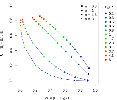
Fig. 2. Mapping different parameterised Mezentsev functions into UW space using Eq. (25). The colours depict certain aridity (Ep/P)
values indicated by the legend in the right.
Figure 2 illustrates the functional behaviour of the Mezentsev function for different catchment parametersnin
UW space. The Budyko functions describe curves in the UW
space, whereby values ofn >1 result in smaller values of both,WandU. Also note that forn= 1 the Mezentsev func-tion Eq. (18) follows the negative diagonal of the climate change hypothesis, cf. Fig. 1.
More important for streamflow change assessment is that the Budyko functions display curves in the UW space. Gen-erally, the derived climate sensitivity is a tangent at some aridity value of a Budyko function. Meaning that there are different climate change directions in UW space (CCD), de-pending on the aridity of a basin and the respective Budyko curve. So, under humid conditions climatic changes are more sensitive on relative excess water (larger change in runoff ra-tio than in relative excess energy). Thus the slope of the tan-gent forn >1 will be larger than -1, but not exceed 0. Under arid conditions changes are more sensitive to relative excess energy and the slope will always be smaller than -1. That means, independent of any given condition (P , E0, n) and any climatic change (1EPp), the slope will always be nega-tive and thus−∞< 1U/1W <0, which refers to change directions into the 2nd (90◦< α <180◦) or the 4th quadrant
(270◦< α <360◦) in Fig. 1. Moreover, it is interesting to note, that ifP=Epthe CCD obtained by the Budyko frame-work using Mezentsev’s curve is identical to the one of the CCUW hypothesis. The differences to the CCUW hypothesis are generally increasing the more humid/arid a given basin is. Further, the larger the catchment parametern, the larger the differences. A mathematical derivation of the climate change direction of the Mezentsev function (αmez) can be found in the Appendix A.
EpP
ET
P
0 1 2 3 4 5
0.0
0.2
0.4
0.6
0.8
1.0
n = 0.5 n = 0.8 n = 1.3
n =CE=1
CE=0.5
CE=0.8
CE=1.3
CCUW Mezentsev water limit
energy limit
Fig. 3. Mapping of CCUW hypothesis into Budyko space for dif-ferent values of catchment efficiency (CE) using Eq. (26). For com-parison different parameterisations of the Mezentsev curve are also shown. The grey lines depict the theoretical limits for water and energy.
3.2 Mapping CCUW into Budyko space
For comparison of the CCUW hypothesis with the estab-lished Budyko functions we map the CCUW hypothesis into Budyko space and visualise the differences. For the purpose of mapping we come back to Eq. (8), whereCEis assumed to
be a constant, which is a consequence of the climate change impact hypothesis in UW space. With that we can rearrange Eq. (8) to achieve a mapping to Budyko space:
ET
P =CE Ep P +Ep
. (26)
Figure 3 illustrates the functional form of change predic-tions of the CCUW hypothesis for different values of CE.
These can be compared with the curves for different parame-terisations of Eq. (18). The curves of the CCUW hypothesis are strongly determined byCE, similar to the effect of
dif-ferent values for the catchment parametern in the parame-terised Budyko model of Mezentsev (1955). By recollecting Eqs. (18) and (26) we can see, that forn= 1 andCE= 1 both
functions are identical.
It is, however, important to note, that there is a different asymptotic behaviour of the CCUW hypothesis compared to the Budyko hypothesis. The actual value of the catchment efficiency CE determines the asymptote for Ep/P→ ∞. This makes a distinction from the Budyko hypothesis, which employs the water limitET/P= 1 as asymptote for
Ep/P→ ∞. Especially under more arid climatic conditions the differences in climatic sensitivity are apparent. When
CE>1, the slopes of the CCUW function are steeper than
[image:6.595.309.547.62.258.2]-1.0 -0.5 0.0 0.5 1.0
-1
0
1
2
3
4
5
ΔP/P
Δ
Q/Q
Sensitivity of Q to P
W = Q/P 0.1 0.3 0.5 0.7 0.9
-1.0 -0.5 0.0 0.5 1.0
-1
.0
-0
.5
0.0
0.
5
1.0
ΔP/P
Δ
ET ET
Sensitivity of ET to P
EpP
0.2 0.6 1 2 4
-1.0 -0.5 0.0 0.5 1.0
-1
0
1
2
3
4
5
ΔEp Ep
Δ
Q/Q
Sensitivity of Q to Ep
W = Q/P 0.1 0.3 0.5 0.7 0.9
-1.0 -0.5 0.0 0.5 1.0
-1
.0
-0
.5
0.0
0.
5
1.0
ΔEp Ep
Δ
ET ET
Sensitivity of ET to Ep
EpP
[image:7.595.120.474.65.423.2]0.2 0.6 1 2 4
Fig. 4. Relative change in response to relative changes inP (top panels) and inEp(bottom panels) ofQ(left panels) andET (right panels)
as predicted by the CCUW hypothesis. Changes inQare dependent on runoff ratioWand on aridityEp/Pand are coloured with respect to
the respective runoff ratio and shown for an aridity index ofEp/P= 1. Relative changes inET are dependent on aridity only and lines are coloured with respect to different aridity indices. Note that changes of1Q/Qsmaller than−1 are not physical.
more levelled. For example, let us consider the case of in-creasing aridity and a basin on the curve for CE= 1.3 as
shown in Fig. 3. At some point the water limit (ET =P)
will be reached, which means that all precipitation is evapo-rated and there is no runoff anymore. Any points on the curve above the water limit violate the water balance, because ac-tual evapotranspiration can not be larger than the water sup-ply. Thus, for physical reasons,CEhas to decrease when
ap-proaching the Budyko envelope. This means that the strong assumption of the CCUW hypothesis with constantCE can
not be valid for all hydro-climatic states and streamflow sen-sitivity results of basins close to the Budyko water and energy limits are probably not realistic.
3.3 Climatic sensitivity of basin evapotranspiration and streamflow
In the theoretical section of this paper we derived analyti-cal equations (i) for predicting the absolute hydrologianalyti-cal re-sponse for variations in climate and (ii) for estimating the climatic sensitivity, i.e. the proportional change inET orQ
by a proportional change in climate.
having a smaller (larger) sensitivity. In the right panels of Fig. 4 the relative changes inET due to relative changes in
P (upper panel) and inEp(lower panel) are shown. The fig-ures highlight that the magnitude of relative change is de-pendent on the aridity of the given basin. So the more arid the climate, the larger are changes inET due to changes in
P, while changes inEpshow the opposite behaviour. In addition, the curves shown in Fig. 4 display substantial nonlinear behaviour to changes either inP orEp. Consider-ing the rainfall-runoff relation, this means that the relative change in streamflow is not proportional to the change in precipitation, but also depends on the magnitude of change in precipitation. In general, positive precipitation changes result in stronger changes in streamflow, than negative pre-cipitation changes. Such features have e.g. been reported by Risbey and Entekhabi (1996), analysing the response of the Sacramento River basin (US) to precipitation changes. While Risbey and Entekhabi (1996) argue that hydrological mem-ory effects are related to this nonlinear behaviour, our anal-ysis suggests that the coupled nature of water and energy balances is the primary cause of the nonlinear response of streamflow to climate.
Next, we discuss and compare climate elasticities de-rived by the CCUW and the Budyko sensitivity approaches. Kuhnel et al. (1991) showed thatεp+εEp= 1. Therefore, we
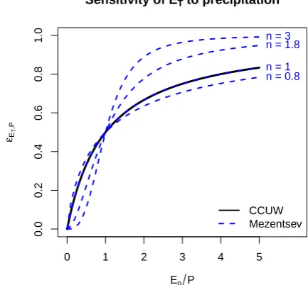
only discuss the elasticity to precipitation. Figure 5 displays the elasticity ofET (εET,P) as a function of aridity. In more
humid or semi-arid conditions (Ep/P <2), the differences between the Budyko function elasticities and the ones de-rived by the CCUW hypothesis are small. In each case the sensitivity increases with aridity. In more arid conditions larger differences of the CCUW hypothesis to the Budyko sensitivity functions become apparent. Thereby, the paramet-ric Budyko function withn >1 approaches the upper limit (εET,P= 1) distinctly faster than the CCUW method.
So for example, a precipitation decrease of 10 % in an arid basin withEp/P= 4 results in an estimated change ofET by
8 %, when the CCUW hypothesis is applied. However, apply-ing the Budyko framework with the Mezentsev function and
n= 1.9,ET changes by 9.3 %. Even though this seems to be
a small difference, in absolute values such changes are large, when considering the fact that in such arid basins annualET
is almost as large as annual precipitation.
Regarding the elasticity of streamflow, the picture gets more complicated. First, the sensitivity of streamflow is also dependent on streamflow itself, cf. Eqs. (17) and (22). Sec-ondly, in arid conditions, streamflow is typically very small compared to all other variables considered here. So even small absolute changes inQmay result in very large elas-ticity coefficients. In Figure 6 we showεQ,P as a function of
aridity. Because of the dependency to streamflow, or rather to catchment efficiency, we plotεQ,P as computed by CCUW
for different values ofCE. The effect ofCEon streamflow is
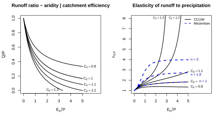
shown in the left panel of Fig. 6, where we plot the runoff ra-tioQ/P as a function of aridity. The streamflow elasticities
Sensitivity of ET to precipitation
Ep P εET
,P
0 1 2 3 4 5
0.0
0.2
0.4
0.6
0.8
1.0
n = 0.8 n = 1 n = 1.8 n = 3
CCUW Mezentsev
Fig. 5. Sensitivity (elasticity) of basin evapotranspiration with re-spect to changes in precipitation (εET,P). The bold black line de-picts elasticity of the CCUW, while the dashed line shows different elasticities for the Mezentsev function. The elasticity of the CCUW corresponds with the slope of the curves shown in the top right panel of Fig. 4.
derived by the CCUW method clearly show for arid condi-tions, that the largerCE(and thus smallerQ), the larger gets
εQ,P. In contrast the elasticities of the Mezentsev functions
converge to a maximal level ofεQ,P=n+ 1 forEp/P→ ∞. 3.4 Climate-vegetation feedback effects
As detailed in the theory section and illustrated above, both, the Budyko functions and the CCUW hypothesis provide an-alytical solutions for the problem of howET orQare
chang-ing whenP orEpare changing. However, there are very dif-ferent outcomes with respect to the determined sensitivity. In the following we discuss the origins and implications of these differences in more detail.
The key difference of the parametric Budyko approach is that the sensitivity of the hydrological response (ET,Q) is
also dependent on changes in the catchment parameter n, cf. Eqs. (21) and (22). In contrast the CCUW approach is only sensitive to changes inP andEp, cf. Eqs. (16) and (17). Thus, it is interesting to study the influence of the catchment parameter encoding catchment properties on hydrological re-sponse under transient climatic conditions. Further, the elas-ticity concept of Schaake and Liu (1989), Eq. (11), shows that the sensitivity coefficients are composed of two compo-nents, which is also apparent in the sensitivity terms within Eqs. (21) and (22).
For the purpose of illustration we conduct the following experiment: we deriveET andQfor different aridity indices
EpP
Q/P
0 1 2 3 4 5
0.0
0.2
0.4
0.6
0.8
1.0
CE=0.8
CE=1 CE=1.1
CE=1.2 CE=1.3
Runoff ratio ~ aridity | catchment efficiency
EpP
εQ,P
0 1 2 3 4 5
1
2
3
4
5
6
7
8
Elasticity of runoff to precipitation
CE=0.8 CE= CE=1.1
CE=1.3 CE=1.2
n = 3
n = 1.8
[image:9.595.125.469.58.240.2]n = 1 CCUW Mezentsev
Fig. 6. Left panel: runoff ratio as a function of aridity for different, but fixed values of catchment efficiency (CE) using Eq. (26). Right panel:
elasticity coefficient of streamflow to precipitationεQ,P as a function of aridity. Displayed are the elasticities derived from the CCUW hypothesis (black for different values ofCE), and the elasticities derived from different parameterisations of the Mezentsev functions using Eq. (22).
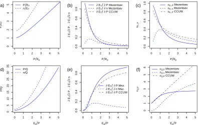
Mezentsev function withnset to 1.8. In Fig. 7 we plot the two components of the sensitivity coefficientsεET,P,εET,n and εQ,P,εQ,nas functions of the humidity indexP /Epand the aridity indexEp/P, respectively. The purpose of the differ-ent x-axes is to highlight the differences in sensitivity, which become apparent forET under humid conditions and forQ
under arid conditions.
The top panels show the sensitivity ofET to P andn,
which can be decomposed intoεET,P=P /ET·∂ET/∂P and εET,n=n/ET ·∂ET/∂n, respectively. Panel a displays the
first terms of these sensitivity coefficients, which are both increasing with humidity. In panel b solutions of the par-tial differenpar-tial terms are displayed for the CCUW hypoth-esis (∂ET/∂P=ET/P EpE+pP) and the Mezentsev function
Eq. (23). The curves of ∂ET/∂P of the Budyko and the
CCUW approach intersect at a humidity index ofP /Ep= 1 and show somewhat larger differences when P /Ep>1.5, whereby the Budyko curve approaches 0 faster than the CCUW curve. Panel c then displays the resulting sensitiv-ity coefficients, which is the product of both terms shown in panels a and b. While the differences between the two ap-proaches must be similar to the ones shown in panel b, we find that the sensitivity ofET to the catchment parameter is
larger than the sensitivity toP whenP /Ep>1.5. The rea-son for this behaviour is mainly due to the first term of the coefficients:n/ET is rising faster thanP /ET (ifn >1).
The lower panels of Fig. 7 are constructed analogously, but display the sensitivity of streamflow as a function of the arid-ity index. From panel d we see that the inverse of the runoff ratio is strongly increasing with aridity, but similar to the panel aboven/Qis rising faster thanP /Q. Panel e is only different from panel b, asP /ET has been switched. It
high-lights that there are larger differences between CCUW and
the Budyko approach, whenEp/P >1.5, which we already discussed with respect to Fig. 5. From panel f, we can see that these differences in∂ET/∂P have large consequences for the
resulting streamflow sensitivities. Whereby,εQ,P;ccuwis pro-portionally increasing withP /QandεQ,P;mezapproaches its maximal level ofn+ 1. Thus, the strong exponential effect of the inverse runoff ratio shown in panel d is heavily reduced. And mirroring the results ofET above, the sensitivity ofQ
to changes in the catchment parameter is strongly increas-ing with aridity and apparently larger than the sensitivity to precipitation in arid basins.
Combining these findings, some important and scientifi-cally interesting conclusions can be made. First, under limit-ing conditions, either a lack of water or a lack of energy, we find an increasing importance of the catchment properties re-flected in the catchment parameter of the parametric Budyko model. Considering the similarities of the Mezentsev func-tion in Eq. (18) and the CCUW hypothesis transformed into Budyko space in Eq. (26), we conclude that the inclusion of the catchment parameter essentially accounts for these limit-ing conditions. This agrees with the mathematical derivation of the Mezentsev function by Yang et al. (2008). Secondly, the inclusion of the catchment parameter results in larger sensitivities of streamflow and actual evapotranspiration to changes in catchment properties than to changes in climate. This can explain the levelled climatic sensitivity of stream-flow under arid conditions even thoughP /Qis strongly in-creasing with aridity.
0 1 2 3 4 5
0
1
2
3
4
5
P Ep
P
ET
P ET n ET (a)
0 1 2 3 4 5
0.0
0.2
0.4
0.6
0.8
P Ep
∂
ET
∂
P
,
∂
ET
∂
n
∂ET ∂P Mezentsev ∂ET ∂n Mezentsev ∂ET ∂P CCUW (b)
0 1 2 3 4 5
0.0
0.2
0.4
0.6
0.8
1.0
P Ep εET
,P
εET,P Mezentsev εET,n Mezentsev εET,P CCUW (c)
0 1 2 3 4 5
0
5
10
15
20
25
30
35
EpP
P/Q
P/Q n/Q (d)
0 1 2 3 4 5
0.0
0.2
0.4
0.6
0.8
EpP
∂
ET
∂
P
,
∂
ET
∂
n
∂ET ∂P Mez. ∂ET ∂n Mez. ∂ET ∂P CCUW (e)
0 1 2 3 4 5
0
1
2
3
4
5
6
EpP εQ,P
[image:10.595.101.497.61.311.2]εQ,P Mezentsev εQ,n Mezentsev εQ,P CCUW (f)
Fig. 7. Sensitivity coefficients and their components as functions of the humidity and aridity index, respectively. Baseline water balance terms (ET andQ= 1−P) have been determined with the Mezentsev function andn= 1.8. For illustration purposes we setP= 1 andEp= 0 ... 5. Top
panels display components of the sensitivity of actual evapotranspirationET to precipitationP and the catchment parameternas functions of the humidity indexP /Epusing terms of Eq. (21). The bottom panels display components of the sensitivity coefficient of streamflowQto P andnas functions of the aridity indexEp/Pusing terms of Eq. (22). The left panels depict the left term of the sensitivity coefficients, the
middle panels the right term (solutions of the partial differentials∂ET ∂n and
∂ET
∂P ) and the right panels show the sensitivity coefficients.
response. Last, the CCUW hypothesis does not lead to such a determined climate-basin characteristic (vegetation) feed-back relation as the Budyko approach. This is most apparent in water limited basins, where the sensitivity of streamflow to changes in aridity derived from the CCUW approach can be much larger than the one derived from the Budyko ap-proach. While the Budyko approach respects the conserva-tion of mass and energy, the CCUW hypothesis may lead to a conflict with the water limit. This indicates that the as-sumptions of the CCUW hypothesis are not applicable under limiting conditions.
4 Application: three case studies
To demonstrate the applicability of the newly derived stream-flow sensitivity method, we selected data of three differ-ent large river basins. We compare the climate sensitivities and absolute streamflow change predictions with the Budyko approaches.
For the case studies we selected the Murray-Darling Basin (MDB) in Australia (Roderick and Farquhar, 2011), the headwaters of the Yellow River basin (HYRB) in China (Zheng et al., 2009), and the Mississippi River Basin (MRB) in North America (Milly and Dunne, 2001). These large basins differ in climate and include arid (MDB), cold and
semi-humid (HYRB) and warm, humid (MRB) climates. All basins have already been subject to climate sensitivity studies. Using hydro-climate data from the above references we derived climate sensitivity coefficients and compute the change in streamflow, given the published trends in climate. All data and computations can be found in Table 1.
4.1 Mississippi River Basin (MRB)
The largest observed trend in climate of the three basins is found for the Mississippi River Basin (upstream of Vicks-burg). In the period from 1949–1997 we find a marked trend towards a more humid climate with an increasing trend inP
and a decreasing trend in evaporative demand (Ep). As one would expect, the observed streamflow increased (26 %) and all predictions are around that magnitude, thus providing ev-idence that climatic variations explain most of the observed change in runoff. The prediction of the Budyko approach is very close to the observed change in runoff. Also the ob-served change direction of1U/1W withα= 304◦is close to the climate change direction derived from the Mezentsev function, withαmez= 310◦.
The CCUW method yields somewhat larger sensitivities
εQ,P, and thus predicts a larger change in streamflow (about
Table 1. Observations and predictions of streamflow change of three case-study river basins, Mississippi River basin (MRB), the headwaters of the Yellow River (HYRB), and the Murray-Darling River Basin (MDB). Data are taken from the respective reference publications. For prediction of streamflow change we compare the CCUW method (1Qccuw) with the sensitivity approach employing
the Mezentsev function (1Qmez). Change direction in UW spaceα,
corresponding with Fig. 1, is computed by Eq. (6). The theoretical climate change direction derived for the Mezentsev function (αmez)
is computed by Eq. (A5).
unit MRB HYRB MDB
area km2 3.0e + 06 1.2e + 05 1.1e + 06
P mm yr−1 835.0 511.6 457.0
Ep mm yr−1 1027.0 773.6 1590.8
Q mm yr−1 187.0 179.3 27.3
Ep/P – 1.2 1.5 3.5
Q/P – 0.22 0.35 0.06
1P mm yr−1 85.4 −21.0 −17.0
1Ep mm yr−1 −17.8 −23.0 21.0
1Q mm yr−1 48.9 −36.2 −5.6
n – 2.00 1.13 1.74
1n – 0.04 0.18 0.06
CE – 1.41 1.08 1.21
1CE – 0.01 0.09 0.00
εQ,P;mez – 2.38 1.71 2.60
εQ,P;ccuw – 2.55 1.74 4.51
1Qmez mm yr−1 50.0 −8.8 −3.2
1Qccuw mm yr−1 56.1 −8.8 −5.7
α ◦ 304 210 135
αmez ◦ 310 134 111
that CE increased by 1 %. This is consistent with the
in-crease in the catchment parameter (1n), where larger values of n indicate largerET. So we can conclude that most of
the changes in streamflow in the MRB can be attributed to the increase in humidity, but the increase in both,nandCE,
indicates that changes in basin characteristics may have con-tributed to increasingET. Note, that the numbers given for
changes in human water use (e.g. dam management, ground-water harvesting) as given by Milly and Dunne (2001), do not significantly change the magnitude in observed and pre-dicted changes.
4.2 Headwaters of the Yellow River Basin (HYRB)
The headwaters of the Yellow River basin are at high alti-tudes (above 3480 m a.s.l.) and thus relatively cold and re-ceive seasonal monsoon precipitation (Zheng et al., 2009). This basin is also different to the others considered here, as the observed decrease in streamflow (−20 %) comparing the periods 1960–1990 and 1990–2000 cannot be explained by
the long term average changes in precipitation and potential evapotranspiration, which almost neutralise each other. As a result, the methods considered here can attribute only 24% of the observed change to climate variations. Further, the change direction in UW space withα= 210◦implies, accord-ing to the concept of Tomer and Schillaccord-ing (2009) (Fig. 1), that the main direction of the observed change is in basin change direction. Both frameworks indicate that the catchment prop-erties have been changing, with significant increases innand
CE over time. The data reported on changes in land cover
fractions before and after 1990 in Zheng et al. (2009) also implicate land-use change. Especially the increase in culti-vated and forested land (above 120 %) at the cost of grassland supports this direction of change towards higher catchment efficiency.
4.3 Murray-Darling River Basin (MDB)
For a more detailed discussion of the case studies, the MDB has been selected. It has the driest climate (Ep/P= 3.5) of all three basins considered. Also the climatic sensitivity coeffi-cients are largest and climate effects on streamflow are ex-pected to be large. We concentrate on the CCUW hypothesis and the parameterised Budyko function approach, a frame-work which was presented by Roderick and Farquhar (2011), especially for the MDB.
Roderick and Farquhar (2011) report long-term average data for the period 1895–2006 and a period of the last ten years 1997–2006. Comparing these periods, the climate shifted towards increased aridity, with less rain (−3.7 %) and increased potential evapotranspiration (1.3 %). The observed decrease in streamflow is−5.6 mm yr−1(−20.5 %).
From Table 1 we see that (i) the elasticity coeffi-cients to precipitation and (ii) the predicted changes in streamflow are quite different between the Budyko and the CCUW approach. When using the Budyko approach, following Roderick and Farquhar (2011), the sensitiv-ity of streamflow to a relative change in precipitation is
εQ,P;mez= 2.6, which is close to the theoretical upper bound of εQ,P;mez= 1 +n= 2.74. Employing data of the climatic changes in the second period we predict a change of
Climatic sensitivity, Mezentsev, % change in Q
% change in P
% change in
Ep
−20 −10 0 10 20
−20 −10 0 10 20
−100
−50
0
50
100
−400 −300 −200 −100 0 100 200 300 400
Climatic sensitivity, CCUW, % change in Q
% change in P
% change in
Ep
−20 −10 0 10 20
−20 −10 0 10 20
−100
−50
0
50
100
150 200
250
300
[image:12.595.129.467.63.216.2]−400 −300 −200 −100 0 100 200 300 400
Fig. 8. Sensitivity plots of streamflow to percent changes of precipitation andEp, estimated for the long term hydro-climatic states of the
Murray-Darling Basin (as given in Table 1). Contour lines depict the percent change in streamflow. Note that changes of1Q/Qsmaller than−100 % are not physical. Left panel: The Budyko framework using the Mezentsev function and Eq. (22) in accordance to Roderick and Farquhar (2011, Fig. 2). Right panel, sensitivity estimation by the CCUW framework Eq. (10).
able to predict the observed change using the changes ofP
andEp only. We also find that α= 135◦, i.e. the observed change is in climate change direction of the CCUW hypoth-esis, with increased aridity resulting in increasedW and re-ducedU with quite similar absolute values. In contrast, the Budyko framework predictsαmez= 111◦, i.e. there is a larger relative change in the energy partitioning than in the parti-tioning of water.
Figure 8 illustrates the differences between the param-eterised Budyko and the CCUW method on climate sen-sitivity. A diagram which may be practically considered for the assessment of future hydrological impacts of pre-dicted changes in precipitation and evaporative demand (Ep) (Roderick and Farquhar, 2011). We see that the contour lines of the estimates by the CCUW method are about two times more dense compared to the contours of Roderick and Farquhar’s approach. This is due to the fact that the sensi-tivity to precipitation is almost twice as large, cf. Table 1. The CCUW method predicts a larger sensitivity, because the sensitivity is mainly determined by the inverse of the runoff ratio, which is very large for the MDB (P /Q= 16.7). How-ever, the result obtained with the CCUW hypothesis should be taken with care, because it is derived by putting the strong assumption that the concept of Tomer and Schilling (2009) and thus the CCUW hypothesis is valid for any given aridity index. Still, with respect to the discussion in Sect. 3.4, the resulting difference in streamflow sensitivity illustrates the impact of the inherent assumptions on the role of climate-vegetation feedbacks in arid environments.
5 Conclusions
This paper is based on a conceptual framework published by Tomer and Schilling (2009), which links shifts in ecohydro-logical states of river basins to shifts in climate and basin
characteristics. The original concept is based on the obser-vation that climate impacts on streamflow produce shifts in the ecohydrological states of relative excess water and rel-ative excess energy, which are orthogonal to shifts induced by land-use or land management changes. Particularly inter-esting is the hypothesis that changes in the supply of water and energy (i.e. changes in the aridity index) lead to distinct changes in the relative partitioning of water and energy fluxes at the surface. According to the climate change hypothesis (CCUW), an increase (decrease) in the ratio of actual evapo-transpiration to precipitation balances with the decrease (in-crease) in the ratio of actual to potential evapotranspiration. A direct consequence of the CCUW hypothesis, is that the sum of both terms, to which we refer to as “catchment ef-ficiency” (CE), is constant. We then utilise the CCUW
hy-pothesis under the assumption that it is applicable for any aridity index, to derive analytical solutions, (i) to predict the impact of variations of the aridity index on evapotranspira-tion and streamflow, and (ii) to assess the climatic sensitivity of river basins. Both issues are of great practical and scien-tific concern.
5.1 Potentials and limitations
To understand the properties and implications of the method for estimating climate sensitivity, a thorough discussion of its properties is needed for different climates, expressed by aridity and different possible hydrological responses.
showed that under such conditions the CCUW hypothesis does not adhere to the water (ET≤P) and energy limits
(ET ≤Ep) proposed by Budyko (1974).
As we show, the effects are largest for the sensitivity of streamflow under arid conditions, where the sensitivity of CCUW tends to increase with the inverse of the runoff ra-tio, while the sensitivity of the Budyko method approaches a constant value. These findings exclude the use of sensitiv-ity estimates derived by the CCUW hypothesis under hydro-climatic conditions being close to the water limit and limits its use compared to the more general approach of Roderick and Farquhar (2011). In contrast to the CCUW sensitiv-ity framework, their Budyko sensitivsensitiv-ity framework respects the conservation of mass and energy even under limiting conditions.
However, our study allows some conclusions on how to use the simple concept of Tomer and Schilling (2009) to sep-arate climate from land-use effects on evapotranspiration and streamflow. First, the concept (Fig. 1) with the diagonals rep-resenting the change directions, is a special case of sensitivity frameworks using the Mezentsev function under the condi-tion that long-term average precipitacondi-tion equals evaporative demand. The catchments considered by Tomer and Schilling (2009) have been close to this condition and therefore the Budyko framework estimates similar attributions. If condi-tions are different, the climate change (and the basin change) directions given in Fig. 1 need a case specific correction. As we have shown, if a rotation of the original concept is applied for correction, the result will depend on the aridity index and the catchment parametern. Generally, whenn >1 and under arid conditions, the climate change direction is corrected to-wards the ordinate in Fig. 1, while under humid conditions the arrows are towards the abscissa.
5.2 Insights on the catchment parameter
We compare our results with a parametric Budyko function, which was first proposed by Mezentsev (1955) and recently was also applied for the problem of streamflow sensitivity by Roderick and Farquhar (2011). Yang et al. (2008), who derived the Mezentsev (1955) equation by mathematical rea-soning, showed that accounting for the water and energy lim-its leads to a catchment specific constant. This catchment pa-rameter has a range of effects, which increase in magnitude under the lack of water or energy.
This has several interesting implications. First, the catch-ment parameter, describing the integral effect of all processes forming the hydrological response of a catchment, influences the sensitivity of catchmentET to climatic changes. For
ex-ample the type of vegetation of a basin can significantly af-fect climatic sensitivity ofET. This was for example shown
for the aerodynamic and canopy resistance parameters in the Penman-Monteith equation (Beven, 1979). Second, the in-fluence of catchment properties is increasing under limit-ing conditions. As we show, the direct sensitivity ofET to
changes in the catchment parameter can be larger than the sensitivity to changes, e.g. in precipitation, under very wet or very dry conditions. This means that a small change in catch-ment properties can have large relative effects on evapotran-spiration in very humid basins, whereas streamflow would be highly affected in arid basins. On the one hand, this relation will complicate the detection of effects of climatic changes on the water budget in limited environments. On the other hand, we expect that catchment ecosystems adapt to tran-sient climatic changes in order to keep their functionality. Such adaptions are likely to have considerable impact on the resulting hydrological response, however, such climate-vegetation feedback relations are not explicitly considered in any of the two frameworks considered here.
5.3 Validation
In this paper we have compared two hypotheses about how streamflow is changing when long-term average precipitation or evaporative demand are changing. Still, both hypotheses need to be tested and validated.
Here, we give only some recommendations. First, there is the necessity to control for catchment property changes, which complicates any attempt of validation. Still, one could try to trace the hydro-climatic states of individual basins through time, hoping for different climatic boundary con-ditions. Possible test setups are, (i) controlled small scale experiments preferably under more extreme climatic con-ditions (humid, semi-arid, arid). Examples are the agricul-tural experiments described by Tomer and Schilling (2009), long-term experimental watershed programs (Moran et al., 2008) or the Long-term Ecological Research project http: //www.lternet.edu/. Another approach is, (ii) the evaluation of large hydro-climate datasets, where the effect of basin changes can be treated statistically. One example has been presented by Renner and Bernhofer (2011), using a large set of river basins in the United States. In parallel, one could use physically based models, where controlling of basin charac-teristics is easy, but difficult to prove as the choice of param-eters evidently effects the resulting sensitivity coefficients.
Independent of the approach taken, we believe that nor-malising observations such as relative excess energy and wa-ter can reveal inwa-teresting relationships of complex data sets. 5.4 Perspectives
Given the significance of vegetation and ecosystems (Donohue et al., 2007) we believe that ecohydrological mod-els and conceptualising such processes at the catchment scale (Klemes, 1983) is of great importance. Inspiring research introduced the role of soils (Milly, 1994; Porporato et al., 2004), the stochastic role of precipitation (Choudhury, 1999; Gerrits et al., 2009) and the role of self-organising princi-ples of catchment ecosystems (Rodriguez-Iturbe et al., 2011) on the mean annual water balance. However, the remaining challenge is to describe their role under transient climatic conditions.
Appendix A
Derivation of the climate change direction in UW space for the Mezentsev function
Consider a Budyko function which expresses the evaporation ratio as a function of the aridity index8=Ep/P and a catch-ment parameternas
ET/P =f (8, n). (A1)
With Eq. (25) we obtained a mapping of f to the UW space. Using the aridity index as8=Ep/P, Eq. (25) can be written as:
W=1−f (8, n) (A2)
U=1− f (8, n)
8 . (A3)
To estimate the climate change direction in UW space (CCD) of some Budyko function at any given8,n, we need to compute the first derivativeU0ofU=g(W, n), whereby
W is obtained by Eq. (A2). Because Eq. (A3) includes both
f (8, n)and8, we need to derive the inverse of Eq. (A1). The analytical solution for Mezentsev’ function Eq. (18) is derived below. First, Eq. (18) can be rewritten as a func-tion off (8, n)byET /P= 1/(18−n)1/n. Next, we obtain
8=f (W, n)through the inverse of the Mezentsev’ function:
8= 1
1 1−W
n
−1
!1n
. (A4)
Then by inserting Eq. (A4) into Eq. (A3) and differen-tiating with respect to W yields a term for CCD of the Mezentsev’ equation:
αmez=g0(W, n)=
(1−W )2n−(1−W )n (A5)
· (1−(1−W )
n)1−2n
(1−W )n
!n1
.
Last, by substitutingW with Eq. (A2) in Eq. (A5) a rela-tion of the CCD as funcrela-tion of8,ncan be obtained.
Acknowledgement. This work was kindly supported by Helmholtz Impulse and Networking Fund through Helmholtz Interdisci-plinary Graduate School for Environmental Research (HIGRADE) (Bissinger and Kolditz, 2008). The first author wants to thank Kai Schw¨arzel (TU Dresden) for bringing the paper of Tomer and Schilling to his attention. Also the lively discussions with Martin Volk (UFZ – Leipzig) encouraged M. R. to develop the the-oretical basis of this paper. Nadine Große (Uni Leipzig) is credited for clarifying some mathematical operations. Kristina Brust (TU Dresden) is gratefully acknowledged for reading and correcting the manuscript. The critical thoughts of Stan Schymanski (editor), Michael Roderick, Ryan Teuling and one anonymous referee greatly helped to improve the manuscript.
Edited by: S. Schymanski
References
Arnell, N.: Hydrology and Global Environmental Change, Prentice Hall, 2002.
Arora, V.: The use of the aridity index to assess climate change ef-fect on annual runoff, J. Hydrol., 265, 164–177, 2002.
Bagrov, N.: O srednem mnogoletnem isparenii s poverchnosti susi (On multi-year average of evapotranspiration from land surface), Meteorog. i Gridrolog., 10, 20–25, 1953.
Beven, K.: A sensitivity analysis of the Penman-Monteith actual evapotranspiration estimates, J. Hydrol., 44, 169–190, 1979. Bissinger, V. and Kolditz, O.: Helmholtz Interdisciplinary Graduate
School for Environmental Research (HIGRADE), GAIA – Eco-logical Perspectives for Science and Society, 17, 71–73, 2008. Budyko, M.: Climate and life, Academic Press, New York, USA,
1974.
Choudhury, B.: Evaluation of an empirical equation for annual evaporation using field observations and results from a biophys-ical model, J. Hydrol., 216, 99–110, 1999.
Donohue, R. J., Roderick, M. L., and McVicar, T. R.: On the impor-tance of including vegetation dynamics in Budyko’s hydrological model, Hydrol. Earth Syst. Sci., 11, 983–995, doi:10.5194/hess-11-983-2007, 2007.
Donohue, R. J., Roderick, M. L., and McVicar, T. R.: Assessing the differences in sensitivities of runoff to changes in climatic conditions across a large basin, Journal of Hydrology, 406, 234– 244, doi:10.1016/j.jhydrol.2011.07.003, 2011.
Dooge, J.: Sensitivity of runoff to climate change: A Hortonian ap-proach, B. Am. Meteorol. Soc. USA, 73, 2013–2024, 1992. Dooge, J., Bruen, M., and Parmentier, B.: A simple model for
esti-mating the sensitivity of runoff to long-term changes in precip-itation without a change in vegetation, Adv. Water Resour., 23, 153–163, 1999.
Fu, B.: On the calculation of the evaporation from land surface, Sci-entia Atmospherica Sinica, 5, 23–31, 1981.
Gedney, N., Cox, P., Betts, R., Boucher, O., Huntingford, C., and Stott, P.: Detection of a direct carbon dioxide effect in continental river runoff records, Nature, 439, 835–838, 2006.
Klemes, V.: Conceptualization and scale in hydrology, J. Hydrol., 65, 1–23, 1983.
Kuhnel, V., Dooge, J., O’Kane, J., and Romanowicz, R.: Partial analysis applied to scale problems in surface moisture fluxes, Surv. Geophys., 12, 221–247, 1991.
Mezentsev, V.: More on the calculation of average total evaporation, Meteorol. Gidrol., 5, 24–26, 1955.
Milly, P.: Climate, soil water storage, and the average annual water balance, Water Resour. Res., 30, 2143–2156, 1994.
Milly, P. and Dunne, K.: Trends in evaporation and surface cooling in the Mississippi River basin, Geophys. Res. Lett., 28, 1219– 1222, doi:10.1029/2000GL012321, 2001.
Milne, B., Gupta, V., and Restrepo, C.: A scale invariant coupling of plants, water, energy, and terrain, Ecoscience, 9, 191–199, 2002. Moran, M., Peters, D., McClaran, M., Nichols, M., and Adams, M.: Long-term data collection at USDA experimental sites for studies of ecohydrology, Ecohydrology, 1, 377–393, doi:10.1002/eco.24, 2008.
Nash, L. and Gleick, P.: Sensitivity of streamflow in the Colorado Basin to climatic changes, J. Hydrol., 125, 221–241, 1991. Ol’Dekop, E.: On evaporation from the surface of river basins,
Transactions on meteorological observations University of Tartu, 4, 200, 1911.
Porporato, A., Daly, E., and Rodriguez-Iturbe, I.: Soil water balance and ecosystem response to climate change, Am. Nat., 164, 625– 632, 2004.
Renner, M. and Bernhofer, C.: Applying a simple water-energy bal-ance framework to predict the climate sensitivity of streamflow over the continental United States, Hydrol. Earth Syst. Sci. Dis-cuss., 8, 10825–10862, doi:10.5194/hessd-8-10825-2011, 2011. Risbey, J. and Entekhabi, D.: Observed Sacramento Basin
stream-flow response to precipitation and temperature changes and its relevance to climate impact studies, J. Hydrol., 184, 209–223, 1996.
Roderick, M. and Farquhar, G.: A simple framework for relat-ing variations in runoff to variations in climatic conditions and catchment properties, Water Resour. Res., 47, W00G07, doi:10.1029/2010WR009826, 2011.
Rodriguez-Iturbe, I., Caylor, K., and Rinaldo, A.: Metabolic princi-ples of river basin organization, P. Natl. Acad. Sci., 108, 11751, doi:10.1073/pnas.1107561108, 2011.
Sankarasubramanian, A., Vogel, R., and Limbrunner, J.: Climate elasticity of streamflow in the United States, Water Resour. Res., 37, 1771–1781, 2001.
Schaake, J. and Liu, C.: Development and application of simple wa-ter balance models to understand the relationship between cli-mate and water resources, in: New Directions for Surface Water Modeling Proceedings of the Baltimore Symposium, 1989. Schreiber, P.: ¨Uber die Beziehungen zwischen dem Niederschlag
und der Wasserf¨uhrung der Fl¨usse in Mitteleuropa, Z. Meteorol., 21, 441–452, 1904.
Teuling, A., Hirschi, M., Ohmura, A., Wild, M., Reichstein, M., Ciais, P., Buchmann, N., Ammann, C., Montagnani, L., Richard-son, A., Wohlfahrt, G., and Seneviratne, S. I.: A regional perspec-tive on trends in continental evaporation, Geophys. Res. Lett., 36, L02404, doi:10.1029/2008GL036584, 2009.
Tomer, M. and Schilling, K.: A simple approach to distinguish land-use and climate-change effects on watershed hydrology, J. Hy-drol., 376, 24–33, doi:10.1016/j.jhydrol.2009.07.029, 2009. Wang, D. and Hejazi, M.: Quantifying the relative contribution of
the climate and direct human impacts on mean annual streamflow in the contiguous United States, Water Resour. Res., 47, W00J12, doi:10.1029/2010WR010283, 2011.
Yang, H. and Yang, D.: Derivation of climate elasticity of runoff to assess the effects of climate change on annual runoff, Water Resour. Res., 47, W07526, doi:10.1029/2010WR009287, 2011. Yang, H., Yang, D., Lei, Z., and Sun, F.: New analytical derivation
of the mean annual water-energy balance equation, Water Re-sour. Res., 44, W03410, doi:10.1029/2007WR006135, 2008. Zhang, L., Dawes, W., and Walker, G.: Response of mean annual
evapotranspiration to vegetation changes at catchment scale, Wa-ter Resour. Res., 37, 701–708, 2001.
Zhang, L., Hickel, K., Dawes, W., Chiew, F., Western, A., and Briggs, P.: A rational function approach for estimating mean annual evapotranspiration, Water Resources Research, 40, W02502, doi:10.1029/2003WR002710, 2004.