www.hydrol-earth-syst-sci.net/16/4675/2012/ doi:10.5194/hess-16-4675-2012
© Author(s) 2012. CC Attribution 3.0 License.
Earth System
Sciences
Climate change effects on irrigation demands and minimum
stream discharge: impact of bias-correction method
J. Rasmussen, T. O. Sonnenborg, S. Stisen, L. P. Seaby, B. S. B. Christensen, and K. Hinsby
Geological Survey of Denmark and Greenland (GEUS), Copenhagen, Denmark
Correspondence to: T. O. Sonnenborg ([email protected])
Received: 21 March 2012 – Published in Hydrol. Earth Syst. Sci. Discuss.: 18 April 2012 Revised: 27 October 2012 – Accepted: 14 November 2012 – Published: 17 December 2012
Abstract. Climate changes are expected to result in a warmer global climate, with increased inter-annual variability. In this study, the possible impacts of these climate changes on ir-rigation and low stream flow are investigated using a dis-tributed hydrological model of a sandy catchment in western Denmark. The IPCC climate scenario A1B was chosen as the basis for the study, and meteorological forcings (precipi-tation, reference evapotranspiration and temperature) derived from the ECHAM5-RACMO regional climate model for the period 2071–2100 was applied to the model. Two bias cor-rection methods, delta change and Distribution-Based Scal-ing, were used to evaluate the importance of the bias cor-rection method. Using the annual irrigation amounts, the 5-percentile stream flow, the median minimum stream flow and the mean stream flow as indicators, the irrigation and the stream flow predicted using the two methods were com-pared. The study found that irrigation is significantly under-estimated when using the delta change method, due to the in-ability of this method to account for changes in inter-annual variability of precipitation and reference ET and the resulting effects on irrigation demands. However, this underestimation of irrigation did not result in a significantly higher summer stream flow, because the summer stream flow in the studied catchment is controlled by the winter and spring recharge, rather than the summer precipitation. Additionally, future in-creases in CO2are found to have a significant effect on both irrigation and low flow, due to reduced transpiration from plants.
1 Introduction
Future climate changes are expected to result in a generally warmer north European climate (IPCC, 2007b). While the yearly precipitation is expected to stay nearly constant or in-crease slightly in the period up to 2100, significant shifts in the temporal distribution of the precipitation are expected to occur, although the expected nature of this shift varies greatly depending on the climate scenario in question (IPCC, 2007a). In any case, climate change is expected to impact all aspects of the hydrological cycle, thereby changing the availability of fresh water.
The use of groundwater for irrigation is widespread in Northern Europe (Siebert et al., 2010), and is expected to be significantly affected by climate changes. Agricultural de-mand for irrigation depends heavily on precipitation, and creasing temperatures may cause evapotranspiration to in-crease, further increasing this demand. However, there are other factors that may affect the irrigation demands, thereby dampening the effects of the climate changes. These include land use changes to fit the future climate and the expected increase in atmospheric CO2, which may decrease the tran-spiration of crops. All these factors, combined with the fact that the scale and nature of the climate changes is uncer-tain, means that assessing future irrigation demands is a complex task.
significant, may harm the local ecosystems and wildlife that depend on the available fresh water.
In Denmark, approximately one third of all abstracted groundwater is used for irrigation (EUROSTAT, 2012). But the requirement for – and use of – irrigation varies greatly within the country, primarily due to differences in near-surface geology. In the western part of the country, where the top soils are dominated by sand, the use of irrigation is essen-tial for agriculture to be feasible, which has translated into a very high degree of irrigation in this region. While only 18 % of the agricultural area in Denmark is equipped for irriga-tion on average (FAO, 2012), almost 50 % of the agriculture in the western part of the country relies on irrigation. This translates into a potentially high impact on the stream flow in the catchment, especially during dry periods.
A number of studies have previously investigated the link between climate changes, irrigation demands and stream flow. Based on a global model for irrigation requirements and the two general circulation models, GCMs, ECHAM4 and HadCM3, D¨oll (2002) predicts an 8–10 % increase in irriga-tion demands for Western Europe in general between 1990 and 2070. Also using a global model, Fischer et al. (2007) found a significant spread in the expected increase in irri-gation demand for a geographic area spanning Western Eu-rope and Turkey. With mitigation of the future greenhouse gas emissions, their model predicted an increase in irrigation demands of 32–42 % from 2000 to 2070. However, without mitigation, increases between 42 and 147 % are expected for the same time span. The large spread found by this study il-lustrates very well the potential that climate change has for impacting irrigation demands, as well as the large degree of uncertainty associated with the issue. Furthermore, global studies such as D¨oll (2002) and Fischer et al. (2007) cannot accurately capture the strong variability of climate changes on a regional scale. For that, more local studies are required. On catchment scale, studies have been carried out in a number of areas across the globe, ranging from North Amer-ica to Brazil, Indonesia and Spain. For example, using a lo-cal model of the Guadalquivir river basin in southern Spain, D´ıaz et al. (2007) found that irrigation requirements would increase by 15–20 % by 2050. van Roosmalen et al. (2009) showed using a distributed hydrological model for a Danish catchment that irrigation may increase by up to 90 % in 2071 compared to the current level. However, this study featured a highly simplified land use description and only utilized the delta change (DC) method for bias correction.
The impact of the method used for adjusting the output from the regional climate models, RCMs, has been tested by a couple of investigations. Yang et al. (2010) used two dif-ferent methods; the delta change method (Hay et al., 2000) and an approach referred to as distribution based scaling (DBS) (Piani et al., 2010). Whereas the delta change method uses the observed data as baseline and adjustment of only the mean is carried out, the DBS method use the RCM re-sults as baseline and adjust the entire frequency
distribu-tion. In contrast to the delta change method, the distribution based scaling method will reproduce the dynamics of the climate model, e.g. inter-annual variability, prolonged peri-ods of drought or number of days with precipitation. The re-sulting bias-corrected climate data were used as input to the rainfall-runoff model HBV to quantify the effects of climate change on three catchments in Sweden. The DBS approach was found to better preserve the future variability of the RCM outputs. Based on comparison of future discharge from the HBV model larger variability in discharge was found using the DBS adjusted data resulting in, e.g. larger extreme dis-charges than the delta change approach. DBS was found to be more sensitive to the projections used and preserved the annual variability from the corresponding climate model pro-jection. In van Roosmalen et al. (2011) the impact of bias-correction method on the response of a distributed hydrolog-ical model was studied. The delta change method was com-pared to the DBS method. When comparing the hydrologi-cal simulations using both methods, only small differences on the hydrological response were found. It should how-ever be noticed that only average quantities such as annual groundwater recharge, mean change in groundwater level or mean monthly river discharge were analysed. The authors recommend that additional work is needed to analyse, e.g. the impact on extremes.
The aim of this study is to assess the effects of downscal-ing methods on the impact of climate changes on irrigation demands and low flow of streams. A transient distributed physical based model is used, in which all the major hydro-logical processes are dynamically coupled. Climate change impacts are quantified using results from the GCM-RCM combination ECHAM5-RACMO2 forced by the SRES cli-mate scenario A1B for the period 2071–2100. Two methods are used for bias correction of precipitation; the Distribution-Based scaling (DBS) method and the Delta Change (DC) method. Furthermore, two methods are applied to account for the effect of increasing CO2-levels on transpiration. Hy-drological model outputs, such as minimum stream flow, as well as yearly irrigation volumes are used as indicators and compared. The novelty of this study lies in the application of detailed gridded land use data and the focus on quantifying the extreme low flow situations, in order to assess the impact of downscaling method in the driest periods of the year.
2 Methods
2.1 Climate data
2.1.1 Observed climate
Observed climate data is available for the time period 1991– 2010. The grid based precipitation data at 10 km resolu-tion produced by the Danish Meteorological Institute (DMI) (Scharling, 1999) was catch corrected using the dynamic ap-proach proposed by Allerup et al. (1997). The Allerup model was developed for unshielded Hellman rain gauges, on which the Danish rain gauge network is based. Catch correction fac-tors are estimated on a daily basis using air temperature, rain-fall intensity, and wind speed to ensure that short-term vari-ation and inter-annual varivari-ations in the catch deficiency are captured. A detailed description of the implementation of the method is available in Stisen et al. (2011). Reference evap-otranspiration (ET) and temperature is based on the national daily 20 km grid data produced by the Danish Meteorolog-ical Institute (DMI). Reference ET is calculated using the Makkink equation adjusted for Danish conditions (Scharling, 2001) given by
ETm=βM0+βM1 1Si
λ(1+γ ) (1)
where ETm is reference evaporation (mm day−1), λ is the latent heat of vaporization (2.465 MJ kg−1), γ is the psy-chrometric constant (0.667 hPa °C−1), ßM0+ ßM1 are em-pirical constants (0 and 7), 1 is the slope of the vapour pressure curve (hPa◦C−1), and Si is global radiation
(MJ m−2day−1).
2.1.2 Climate model projections
Projected climate comes from the EU project ENSEMBLES, which pairs multiple GCMs (global circulation models) and RCMs (regional climate models) to generate a matrix of tran-sient climate change simulations for the European region (Christensen et al., 2009). The ENSEMBLES project focuses on the A1B emissions scenario as formulated by the UN In-tergovernmental Panel on Climate Change (IPCC) in their fourth assessment report (IPCC, 2007b). This scenario con-tains a more integrated world, with a rapid economic growth and a quick spreading of new technology as well as signifi-cant convergence in income and way of life between regions. In the A1B scenario, the global population and the global emission of greenhouse gasses are expected to peak approx-imately in 2050, after which it will decline. It is very much a mid-severity scenario, in the sense that it predicts a moder-ate increase in the emission of global greenhouse gasses and thus positions itself in between the other scenarios described in IPCC (2007b). For this reason, as of 2010, the Danish Ministry of Climate and Energy is recommending that Dan-ish municipalities use the A1B scenario as a basis for their climate adaptations.
We use one model pairing from ENSEMBLES, based on the ECHAM5 GCM developed by the Max Planck Institute for Meteorology (MPI), and the RACMO2 RCM developed
by the Royal Netherlands Meteorological Institute (KNMI) as we found ECHAM5-RACMO2 to be a median model of climate change for the Danish region. The “future” scenario in this study refers to the far future period 2071–2100. This period was chosen, rather than a period closer to the present, because the change in the climate is expected to be more pro-nounced at the end of the 21st century, meaning that actual climate changes are more distinguishable from natural inter-annual variability in the climate models (Bates et al., 2008).
From the RCM we get direct outputs of including precip-itation (P ) and temperature (T ) at 2 m above ground, and the variables needed for calculating ETref(temperature min-imum and maxmin-imum, incoming long and short wave solar radiation, relative humidity, and wind speed) all on a 25 km grid over a common European region. Actual evapotranspi-ration (ETact) is a direct RCM output, but the simplified representation of land-surface processes including irrigation which is not accounted for makes ETactvalues inadequate as hydrological modelling inputs. Therefore, it is common prac-tice to apply the socalled PET approach to estimate ETact us-ing empirical formulas and output variables from the RCMs (van Roosmalen, 2009; Ekstr¨om et al., 2007).
ETref is estimated using the FAO Penman-Monteith equation (Allen et al., 1998) and RCM output:
ETp=
0.4081(Rn−G)+γT900+273u2(es−ea)
1+γ (1+0.34u2)
(2)
where ETpis the reference evapotranspiration (mm d−1),Rn is the net radiation at the crop surface (MJ m2d−1),T is the mean daily temperature at 2 m height (◦C),u
2 is the wind speed at 2 m height (m s−1),e
s–ea is the saturation vapour
pressure deficit (kPa),1is the slope of the vapour pressure curve (kPa °C−1), andγ is the psychrometric constant (kPa °C−1). Note that this description of the reference ET refers to a hypothetical reference crop with a height of 0.12 m, a surface resistance of 70 s m−1, and an albedo of 0.23.
RCMs have a systematic wet bias resulting in low inten-sity precipitation on a high number of days, which is com-monly corrected so the frequency of dry days in the climate model reference period is equivalent to the frequency in the observations (Gutowski et al., 2007). On a seasonal basis, we calculate a cut-off value in the RCM reference period corre-sponding to the realistic percentage of dry days in the ob-servations, and correct data both within and outside of the reference period, where values below the cut-off are set to zero. Finally, T, dry-day corrected P, and estimated ETref are interpolated from the 25 km ENSEMBLES grid to the corresponding 10 km observational climate grid.
the Distribution-Based scaling method (Piani et al., 2010) are used to generate future climate forcing data.
The delta change (DC) method consists of simply per-turbing baseline climatic data using monthly change factors which are calculated from the differences in atmospheric out-put from the RCM for the current climate and the scenario (future) period. Using the DC method, a historic 20 yr time series, from 1991 to 2010 (here denoted “current”), of me-teorological data (precipitation, reference ET and tempera-ture) are perturbed to emulate the 30 yr future period 2071– 2100. For flux variables (P and ETref)relative change fac-tors are applied, whereas for the state variableT, absolute change is applied. The DC method for precipitation can be formulated as
P1(i, j )=1P(j )·Pobs(i, j );i=1,2, . . . .31;
j=1,2, . . . .12 (3)
where P1 is the precipitation after perturbation using the
change factor (i.e. the input to the hydrological model) and Pobsis the observed precipitation in the historic period. The suffixesiandj stand for the day and the month, respectively. 1P is the DC factor which is calculated as follows
1P(j )=
Pfuture(j ) Pcurrent(j )
;j=1,2, ...,12 (4)
whereP (j )is the precipitation for thejth month, averaged for the entire period of either the future or the current sce-nario. The same method is used for ETref, while temperature bias correction is based on the absolute change and thus the DC method can be formulated as:
T1(i, j )=Tobs(i, j )+1T(j );i=1,2, . . . .31;
j=1,2, . . . .12 (5)
where the DC factor,1T, is defined as
1T(j )=Tfuture(j )−Tcurrent(j ). (6) Distribution based scaling (DBS) is an emerging bias correc-tion method for precipitacorrec-tion that preserves mean amounts and also scales based on daily intensity. The DBS method has been implemented and well documented for precipita-tion over Europe (Piani et al., 2010), Sweden (Yang et al., 2010), and Denmark (van Roosmalen et al., 2011). Unlike the DC method, which only transfers mean changes, the DBS method is able to capture projected changes in the entire pre-cipitation regime, including changes in mean, variability, fre-quency, and intensity.
A gamma distribution provides a good theoretical repre-sentation of precipitation intensity, as well as other meteoro-logical variables that are asymmetrical and positively skewed (Wilks, 2005). The gamma distribution is defined by two pa-rameters, the shape parameter alpha (α)and the scale param-eter beta (β). On a seasonal basis a PDF of the gamma dis-tribution is first fit to dailyP (mm) in the observations data
set, then to the RCM data in same reference period, and fi-nally, future RCM precipitation is corrected using the gamma distributions from the two data sets. Initially, there was diffi-cultly capturing variance in the observed precipitation, sug-gesting that extreme values (upper and lower tails) cannot be represented with a single gamma distribution. Therefore, a double gamma distribution split at the 95th percentile is used similar to Yang et al. (2010). Ultimately, there are two sets of parameters describingPabove and below the 95th percentile for the observations and the RCM, which are used to correct RCM daily futureP according to the following method: Pcorr=f−1(αobs, βobs, f (αctrl, βctrl, PRCM)) (7) wherePcorris the bias corrected RCM dailyP in the past and future periods,f is the PDF of the gamma distribution, and f (αctrl,βctrl, PRCM)is the probability of the valuePRCM esti-mated from the PDF fitted to the RCM control period gamma distribution. ETreffor the current climate was not able to fit a single or double gamma distribution, therefore, a monthly error bias method was used on T and ETref since they are closely tied.
2.1.3 Scenarios
In this study four model scenarios are considered: current, current DBS, DC and DBS. The current scenario refers to the period 1991–2010 in which observed climate data has been used as model forcing. In the current DBS scenario, the DBS corrected climate data from the ECHAM5-RACMO2 has been used for the period 1981–2010 and in the DBS sce-nario the DBS corrected ECHAM5-RACMO2 data has been used for the future period (2071–2100). Finally in the DC scenario, the DC factors for the future period has been ap-plied to the observed data to obtain a 20 yr data series rep-resenting 30 yr statistically. The current scenario thus forms the basis for evaluating climate changes with the DC method as the current DBS scenario does for the DBS method. 2.2 Evapotranspiration and CO2
Experimental studies have shown that rising CO2levels will lead to a reduction in evapotranspiration as the stomatal opening of plants is reduced (Medlyn et al., 1999; Krujit et al., 2008). This will lead to a higher water use efficiency in crops, reducing the need for irrigation making a larger frac-tion of precipitafrac-tion available for runoff and recharge, thus mitigating the effects of the reduced summer precipitation.
Potential ET (ETP)is commonly calculated from reference ET (ETref)using a vegetation specific crop factor,kc(Allen et al., 1998)
ETP=kc·ETref. (8)
To account for the CO2-effect, Krujit et al. (2008) proposes the introduction of a CO2dependent, vegetation specific cor-rection factor,c:
ETP=c·kc·ETref. (9)
The correction factor is a product of three factors related to the stomatal conductance, boundary-layer properties and transpiration share of the total evapotranspiration, respec-tively:
c=Sgs·ST·FT ·1CO2 (10)
where Sgs(ppm−1)is the sensitivity of crop conductance,gs, to CO2:
Sgs=(dgs/gs)/dCO2 (11)
ST (-) is the relative sensitivity of transpiration,T, to crop
conductance:
ST =(dT /T )/(dgs/gs) (12)
and FT is the transpiration share of evapotranspiration
(T/ET).
Sgsis in Krujit et al. (2008) estimated using observed ef-fects of CO2 increases on gs. Based on a literature review of publications where the decrease in gs due to CO2 has been determined experimentally, they found that for grass and herbal cropsgsis−0.093 %.
ST is in the same publication estimated from results
pre-sented by Jacobs and De Bruin (1992) where a process-based model of transpiration is coupled to a model for the atmo-spheric boundary layer to model the interaction between veg-etation and the atmosphere. Using this method,ST is
esti-mated at 0.15–0.20 for smooth surfaces such as grass and 0.40–0.75 for rough surfaces, such as forest. Using these val-ues as reference points,ST for the different crop types were
estimated at Grass 0.175 (throughout the year), wheat and barley 0.3 (summer) and 0.1 (winter), and maize 0.35 (sum-mer) and 0.2 (winter).
Finally, FT is derived using the SWAP
(Soil-Water-Atmosphere-Plant) model (van Dam et al., 2008). Here,FT
is estimated at 0.8 for grasslands (constant throughout the year) as well as 0.8 (summer) and 0.1 (winter) for agricul-tural fields.
The applied change in CO2 concentration (1CO2) is found as the increase in CO2 concentration from 2010 (391 ppm) to the average concentration for the period 2071– 2100 (665 ppm for the A1B scenario) (IPCC, 2011).
The correction factor was found by averaging the calcu-lated CO2concentration for the future scenario (2071–2100),
and applying Eq. (9). This yielded correction factors of 0.96 (grass), 0.94 (wheat and barley), and 0.91 (maize). Note that only the summer correction factors were used, as the winter ET is insignificant.
2.3 Hydrological model
The hydrological model used in this study is a transient, spa-tially distributed groundwater-surface water model based on the MIKE SHE code (Abbot et al., 1986). This model code was chosen primarily due to the possibility for detailed de-scription of the irrigation in the model domain, but also for the comprehensive description of the feedback between the hydrological processes. The groundwater is modelled using a three-dimensional, finite difference model coupled with a simplified linear unsaturated zone model (Yan and Smith, 1994). Evapotranspiration is modelled using the formulation by Kristensen and Jensen (1975). Stream flow is modelled using the MIKE 11 code, dynamically coupled with MIKE SHE, with a kinematic routing description.
2.3.1 Irrigation description
Irrigation is described using the so-called “single well” op-tion (DHI, 2011), where water abstracted at a given locaop-tion is applied to the surrounding area of that well. Well locations and filter depths available from the national well database Jupiter are used as input. The irrigated area for each well is based on reported areas from the municipalities of the area, where such data exist (approx. 70 % of the irrigated area of the model domain), while the remaining 30 % is simply de-fined by a circle with a radius of 400 m around each irrigation well, within which irrigation can take place.
Numerically, irrigation is described using a demand driven scheme. Demand is calculated using the maximum allowed deficit method, where irrigation is started and stopped at user specified soil moisture deficit values. The available water for crop transpiration (AW) is defined as
AW=θ−θwilting (13)
whereθis the actual moisture content andθwiltingis the mois-ture content at the wilting point for the root zone. However, the transpiration is corrected to account for the reduction of root water uptake and transpiration that occurs at lower mois-ture deficit. In the model, this is included by reducing the transpiration linearly from when the AW is a fraction of 0.75 of the maximum available water content (MAW) to the wilt-ing point. Thus, transpiration will occur at the maximum rate until this fraction is reached. Then the transpiration will de-crease linearly until the wilting point is reached, at which point transpiration becomes zero. The MAW is defined as
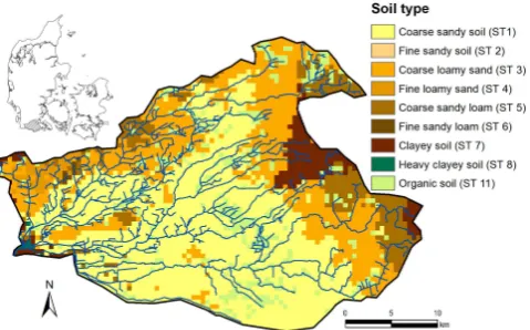
Fig. 1. Map showing the distribution of soil types in the catchment.
whereθfieldis the moisture content at field capacity. The soil moisture deficit (SMD) is thus defined as
SMD=MAW−AW
MAW . (15)
In this study, the SMD-stop value, i.e. the SMD at which irrigation is stopped, is kept constant throughout the year, while the SMD-start value is set to 1 in the winter, implying no irrigation, and a value between 1 and the stop value in the summer to allow for irrigation to take place. These start and stop values were included in the calibration of the model, due to the impact of these values on the irrigation amount and temporal distribution.
2.3.2 Land use parameterization
Land use parameterization for each of the land use types are derived using the soil-plant-atmosphere model DAISY (Sty-czen et al., 2004). Based on climate data and soil charac-teristics the seasonal development in leaf area index (LAI), crop coefficient (kc)and root depth (RD) are produced by DAISY. While grass, paved areas, and needle leaf forest are described using constant parameters throughout the year, all other land use types are divided into a growing season (GS) and a non-growing season, and thus described using time-dependent parameters.
3 Study area
3.1 Geography
The study area is located in the southern part of the Jutland Peninsula in western Denmark (Fig. 1). The area includes the upstream part of the Vidaa River catchment with an area of approx. 850 km2. The topography of the area displays a gentle sloping from the east (approx. 70 m a.s.l.) to the west (approx. at sea level). The catchment is bounded to the east by the Jutland Ridge and by local water divides to the north,
south, and east. The area is largely rural, with only a few small towns present, the two biggest being Rødekro (popu-lation 6000) and Tinglev (popu(popu-lation 2800). The catchment is intensely farmed and has a high degree of irrigation. The catchment is well monitored in terms of stream discharge, ir-rigation amounts and groundwater hydraulic head, and there-fore forms a good platform for assessing the impact of cli-mate change on stream flow and irrigation demands. 3.2 Geology and soil characterization
The location of the main ice border of the Weichselian glacia-tion divides the upper sequence of the Quaternary deposits of Jutland into an eastern part with mainly clayey and sandy tills and a western part dominated by melt water sand and gravel. The Vidaa River catchment is primarily located to the west of the main ice border. Marine inter-glacial sandy clay deposits are also present in the Quaternary sequence of the western part of the area. The thickness of the Quaternary deposits varies largely (Sonnenborg et al., 2003). Miocene sediments are found directly below the Quaternary deposits. The Miocene sedimentary sequence is dominated by shal-low marine to lacustrine and fluvial deposits. The sequence is formed by layers of mica clay, silt and sand together with quartz sand and gravel. The thickness of the deposits varies from few meters to over 200 m from east to west. Generally, the Miocene sediments are assumed to be coarser to the east (Harrar and Henriksen, 1996). Thick clay layers of Eocene and Paleocene age are situated below the Miocene sediments. These formations are assumed to act as impermeable bound-aries to flow and are therefore not included in the model.
The geological model used in this study is predominantly based on lithological information from water supply and oil exploration boreholes in combination with geophysical surveys. The subsurface was described using five different hydrofacies: quaternary sand and clay, and Pre-Quaternary mica sand, mica clay, and quartz sand.
Based on texture data the topsoil is described using nine soil types (Greve et al., 2007), Fig. 1. Spatially distributed maps of soil hydraulic properties by Greve et al. (2007) are used to estimate average values of field capacity and wilting point for each soil type (Table 1).
3.3 Climate and hydrology
Table 1. Soil type (ST) parameters.
Soil description θfield(-) θwilting(-)
Coarse sandy soil (ST 1) 0.16 0.02 Fine sandy soil (ST 2) 0.18 0.02 Coarse loamy sand (ST 3) 0.21 0.04 Fine loamy sand (ST 4) 0.24 0.05 Coarse sandy loam (ST 5) 0.26 0.07 Fine sandy loam (ST 6) 0.28 0.08 Clayey soil (ST 7) 0.31 0.10 Heavy clayey soil (ST 8) 0.49 0.20 Organic soil (ST 11) 0.34 0.10
precipitation is greatly influenced by convective rain events. As a result, the most intense precipitation events generally occur from June to August, with rainfall intensities typically reaching up to 30–40 mm per day. The average annual tem-perature is 8.7◦C, with a maximum of 16.9◦C in August and a minimum of 1.8◦C in January. Mean reference ET in the area is approximately 565 mm per year (calculated using the Makkink equation adjusted for Danish conditions). Due to predominantly sandy soils in the area and low rainfall inten-sities, overland flow is limited. Hence, the majority of the net precipitation in the area recharges the groundwater sys-tem and leaves the catchment through the streams which are primarily fed by groundwater and drainage flow.
3.4 Land use
Based on data from the local authorities, land use (Fig. 3) is divided into four categories: Grass (21 % of the total area), forest (6 %), paved (2 %), and the dominating agriculture (78 %). The agriculture is divided into four subcategories; winter wheat, summer barley, grass, and maize. Grass and barley are the most common crops at 33 % and 31 % of the to-tal agricultural area, respectively, followed by wheat (21 %) and maize (16 %). Parameterization of the individual land use types are given in Table 2.
4 Model setup and calibration
The model domain used in this study (i.e. the Vidaa River catchment) is a sub-catchment of the Danish national water resource model (the DK-model), and the model setup is sim-ilar to the setup of the DK-model. For a detailed description of the DK-model construction, see Henriksen et al. (2003), Sonnenborg et al. (2003), and Stisen et al. (2012). The model domain is delineated at the groundwater divides, which are identified using the DK-model of which the Vidaa River catchment is a subset. All boundaries are specified with a zero-flux boundary condition.
[image:7.595.70.266.81.205.2]A 200 m grid is used for the horizontal discretization and the groundwater zone is described by 10 computational lay-ers. The geological model is voxel based, using voxels with a
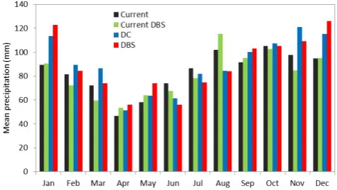
Fig. 2. Mean monthly precipitation in the Vidaa catchment for the current climate, as well as for the future period using both the DC method and the DBS method respectively.
horizontal extent of 1×1 km and a thickness of 10 m. Each geological voxel is assigned a geological unit based on the geological model for the area.
4.1 Calibration
The calibration scheme used in this study is based on the PEST optimization software (Doherty, 2004), which is a commonly used, model-independent nonlinear estimator. Similar to the DK-model calibration (Henriksen et al., 2003), the Gauss-Marquadt-Levenberg local search optimization scheme is used to optimise the parameters of the Vidaa catch-ment model. The basic setup of the calibration scheme is almost identical to the comprehensively described setup of Stisen et al. (2011), in which an adjacent catchment area was modelled using a similar model code and with com-parable data availability. The reader is therefore directed to this publication for a more detailed description of the calibration approach.
A total of 28 parameters are included in the optimization, of which 8 are free and the remaining 20 are tied to the 8 free parameters at a fixed ratio (Table 3). The free parame-ters for calibration are chosen based on a sensitivity analysis. The ratios between the individual tied parameters and free parameters are fixed at the ratios between the initial values of the same parameters.
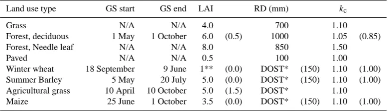
Table 2. Growing season (GS) for each land use type in the model as well as leaf area index (LAI), root depth (RD), and crop coefficient (kc). Values in parenthesis indicate the value of the parameter outside the GS (if different from the parameter value in the GS).
Land use type GS start GS end LAI RD (mm) kc
Grass N/A N/A 4.0 700 1.10
Forest, deciduous 1 May 1 October 6.0 (0.5) 1000 1.05 (0.85)
Forest, Needle leaf N/A N/A 8.0 850 1.50
Paved N/A N/A 0.5 100 1.00
Winter wheat 18 September 9 June 1** (0.0) DOST* (150) 1.10 (1.00) Summer Barley 5 May 20 July 5.0 (0.0) DOST* (150) 1.10 (1.00) Agricultural grass 10 April 10 October 5.0 (1.5) DOST* 1.10 Maize 25 June 1 October 3.5 (0.0) DOST* (150) 1.10 (1.00)
* Parameter is included in the calibration of the model (Table 3). ** LAI is 5.0 for the last two months of the GS. DOST=Dependent on Soil Type (see Table 3).
Table 3. Initial and optimised parameter set as a result of model calibration using PEST.
Parameter Control/Tie Initial value Optimised value Parameter description
Kx, s Free 5.33×10⁻⁴ 5.13×10⁻⁴ Horizontal conductivity, Sand (m s−1) Kx, C Free 2.51×10⁻⁷ 1.20×10⁻⁷ Horizontal conductivity, Clay (m s−1) Kx, QS Free 2.08×10⁻⁴ 4.24×10⁻⁴ Horizontal conductivity, Quartz-sand (m s−1) Kx, GS Free 5.35×10⁻⁴ 6.55×10⁻⁴ Horizontal conductivity, mica sand (m s−1) Drain Free 1.00×10⁻⁷ 7.10×10⁻⁸ Drain time constant (s−1)
Leak Free 1.38×10⁻⁵ 2.76×10⁻⁶ River leakage coefficient (m s−1)
RD, WW1 Free 400 403 Root depth, Winter Wheat, Soil type 1 (mm) SMDst Free 0.60 0.61 Soil moisture deficit for irrigation start (–) Kz, S Kx, s 5.33×10⁻⁵ 5.13×10⁻⁵ Vertical conductivity, Sand (m s−1) Kz, C Kx, C 2.51×10⁻⁸ 1.20×10⁻⁸ Vertical conductivity, Clay (m s−1) Kz, QS Kx, QS 2.08×10⁻⁵ 4.24×10⁻⁵ Vertical conductivity, Quartz-sand (m s−1) Kz, GS Kx, GS 5.35×10⁻⁶ 6.55×10⁻⁶ Vertical conductivity, Glimmer-sand (m s−1) RD, WW2 RD, WW1 600 605 Root depth, Winter Wheat, Soil type 2 (mm) RD, WW3 RD, WW1 800 806 Root depth, Winter Wheat, Soil type 3–4 (mm) RD, WW4 RD, WW1 1000 1008 Root depth, Winter Wheat, Soil type 5–11 (mm) RD, SB1 RD, WW1 400 403 Root depth, Summer Barley, Soil type 1 (mm) RD, SB2 RD, WW1 530 534 Root depth, Summer Barley, Soil type 2 (mm) RD, SB3 RD, WW1 730 736 Root depth, Summer Barley, Soil type 3–4 (mm) RD, SB4 RD, WW1 930 937 Root depth, Summer Barley, Soil type 5–11 (mm) RD, GR1 RD, WW1 400 403 Root depth, Agr. grass, Soil type 1 (mm) RD, GR2 RD, WW1 470 474 Root depth, Agr. grass, Soil type 2 (mm) RD, GR3 RD, WW1 532 536 Root depth, Agr. grass, Soil type 3–4 (mm) RD, GR4 RD, WW1 600 605 Root depth, Agr. grass, Soil type 5–11 (mm) RD, MZ1 RD, WW1 400 403 Root depth, Maize, Soil type 1 (mm) RD, MZ2 RD, WW1 600 605 Root depth, Maize, Soil type 2 (mm) RD, MZ3 RD, WW1 800 806 Root depth, Maize, Soil type 3–4 (mm) RD, MZ4 RD, WW1 1000 1008 Root depth, Maize, Soil type 5–11 (mm) SMDend SMDst 0.40 0.41 Soil moisture deficit for irrigation end (–)
The optimised parameter estimates (Table 3) all fall into realistic ranges and are considered to be reliable.
4.2 Evaluation of model performance
Evaluation of the model performance is based on the Nash-Sutcliffe coefficient,R2NS, and the yearly irrigation amounts. The model shows a good performance for the two stations
[image:8.595.87.509.262.599.2]Fig. 3. Land use in the catchment.
Fig. 4. Observed and simulated yearly irrigation.
catchments in the summer months. This is underlined by the RNS2 calculated for the summer months (0.15, 0.72, 0.83, and 0.91 for the four stations, respectively), and by visual inspec-tion of the hydrographs which showed a good performance with regards to low flow, but difficulties in capturing peak flows.
[image:9.595.45.289.211.411.2]The observed and simulated irrigation amounts are pre-sented in Fig. 4. The model has a tendency to slightly un-derestimate the yearly irrigation, as the mean of the mod-elled yearly irrigation is 23 mm compared to the observed 25 mm. This tendency is particularly clear in years with rela-tively high amounts of irrigation (e.g. 1995–1997). The year 1992 was a particularly dry year, which explains the mod-elled high irrigation amount, and it is likely that the observed amount for that year is lower than the actual irrigation. The data on irrigation is based on voluntary registrations from the farmers and the uncertainty on these data is estimated to be relatively high. Hence, the match presented in Fig. 4 is considered satisfactory.
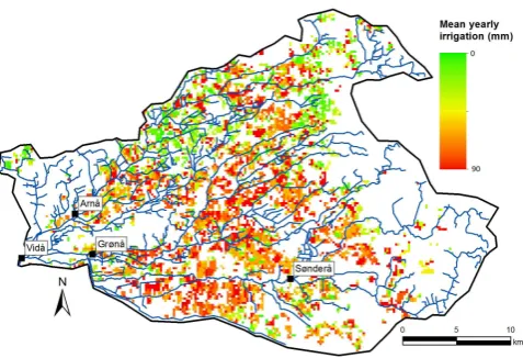
Fig. 5. Mean yearly irrigation (current scenario) in the model do-main and the locations on the stream network where discharge is extracted.
5 Results
The impact of climate change on irrigation and low stream flow are evaluated primarily based on model outputs of mean and maximum yearly irrigation, as well as mean stream flow, minimum flow and median minimum flow, where the lat-ter is defined as the median of annual minimum daily dis-charge. While the irrigation amounts are defined as irrigation (in mm) on the agricultural areas, the stream flow values will be presented for four stations on the stream network (Fig. 5). Station Vid˚a is located at the most downstream point of the stream network, and as such integrate over the entire model domain. Arn˚a station is located on the northern branch of the stream network, with a catchment that is characterized as moderately irrigated. Grøn˚a station is located on the mid-dle (eastern) branch of the network with a catchment that is heavily irrigated. Finally, Sønder˚a station is located on the southern branch, with a catchment that is significantly less irrigated than both the Grøn˚a and Sønder˚a catchment.
To isolate and clarify the effects of bias correction method on the expected climate changes, the results for the future scenario obtained using the DBS data (i.e. the DBS scenario) is compared to the current results also using the DBS data (i.e. the current DBS scenario). Likewise, the results obtained using the DC data (i.e. the DC scenario) is compared to the results obtained using the observed climate data (i.e. the current scenario).
5.1 Comparison of climate data
Table 4. Precipitation and reference ET in the Vidaa catchment area for the current and the future scenario, using the DC method and the DBS method respectively. Note that the term “summer” is in this study defined as the months of May, June, July, and August.
Current Current DBS DC DBS
[image:10.595.248.545.93.388.2]Mean yearly precipitation (mm day−1) 2.74 2.68 2.95 2.93 5 % yearly precipitation (mm day−1) 2.08 2.19 2.24 2.36 Average precipitation stdv (mm day−1) 0.39 0.36 0.41 0.45 Mean yearly reference ET (mm day−1) 1.55 1.62 1.70 1.79 95 % yearly reference ET (mm day−1) 1.66 1.76 1.83 2.17 Mean yearly reference ET stdv (mm day−1) 0.08 0.10 0.09 0.20 Mean summer precipitation (mm day−1) 2.63 2.66 2.39 2.37 5 % summer precipitation (mm day−1) 1.81 1.62 1.66 1.17 Summer precipitation stdv (mm day−1) 0.57 0.66 0.53 0.75
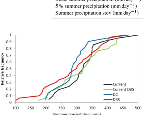
Fig. 6. Cumulative histogram of the summer precipitation for the current climate and for the DC method and the DBS method.
shown. The mean yearly reference ET of the current DBS is 1 % higher than current while the 95-percentile refer-ence ET is 6 % higher than for the observed data. Overall, the current DBS data match the statistics of the observed data satisfactorily.
The mean annual precipitation and reference ET in the Vi-daa River catchment increase slightly when comparing the future climate to the current, as seen in Table 4. This trend is similar using both the DC and the DBS method, although the variability in reference ET is higher for the DBS method. The 5-percentile yearly precipitation for both the DC and the DBS method increases by 8 %, compared to the current and current DBS 5-percentile yearly precipitation. While the mean summer precipitation is expected to decrease by 9 % and 11 % in the DC and the DBS method, respectively, the 5-percentile summer precipitation highlights the difference between the two bias correction methods. The DC method predicts a decrease in the 5-percentile summer precipitation of only 8 %, while a decrease of 28 % is found for the DBS method. This difference is also reflected in the standard de-viation of the summer precipitation, which is significantly higher for the DBS method than for the DC method, illustrat-ing that the inter-annual variation in summer precipitation is
Fig. 7. Cumulative histogram of the number of dry days per summer for the current scenario as well as for the future scenario (DC and DBS methods, respectively).
significantly higher when the DBS method is used. A further inquiry into the temporal distribution of precipitation reveals that while the mean summer precipitation is almost similar in the DC and the DBS method, the DBS method predicts sig-nificantly drier summers than the DC method and a higher frequency of dry summers (Fig. 6). The DBS method pre-dicts that approx. 25 % of summers will see less than 200 mm of precipitation, as opposed to 5 % predicted using the DC method.
[image:10.595.46.290.191.388.2]Table 5. Irrigation indicators for the current scenario and the future scenario using both DC and DBS bias correction.
Current
Current DBS DC DBS
Mean yearly irrigation (mm) 25 32 32 45
95 % irrigation (mm) 49 46 58 95
Yearly irrigation stdv (mm) 12 15 14 28
method, as it is not able to modify the number of dry days since the future precipitation is simply found as a fraction of the current precipitation.
5.2 Irrigation
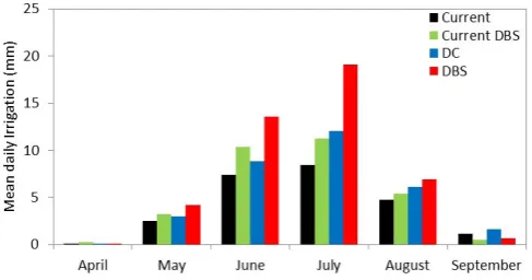
The irrigation indicators are presented in Table 5. Irrigation amounts are predicted to increase in the future for both meth-ods. The mean yearly irrigation increases by 7 mm (31 %) using the DC method and 13 mm (40 %) using the DBS method. The difference between the correction methods is even more pronounced when looking at the 95-percentile yearly irrigation, which increases by 9 mm (18 %) and 49 mm (106 %) for the DC and the DBS methods, respectively. The discrepancies between the results obtained using the two methods suggest that while the DC method may reproduce the mean climate satisfactorily, it is not able to include the change in inter-annual variability of these factors nor the change in dynamics within the year. This is further under-lined by the results on the 95-percentile and standard devia-tion of the irrigadevia-tion, both of which are significantly higher for the DBS method than for the DC method. In Fig. 8 the cumulative distributions for annual irrigation amounts show that while the DC method only results in a shift to slightly higher irrigation amounts compared to the current climate, the curve for DBS has a significantly different shape with much higher irrigation values, especially at high frequencies. Figure 9 reveals that the basic bell shaped distribution with the bulk of irrigation taking place in June and July is similar in both the current and the future scenario. In the current sce-nario, 65 % of the yearly irrigation takes place in June and July, while the corresponding values for the future scenario are 66 % (DC) and 73 % (DBS).
5.3 Stream flow
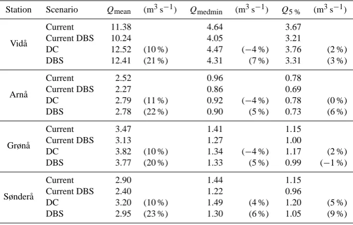
[image:11.595.49.285.92.158.2]In order to differentiate between the effects of climate change alone and the additional effects of changes in irrigation, two scenarios were carried out with the hydrological model where irrigation initially was inactive and active in subse-quent simulations. In Table 6, mean, median minimum and 5-percentile discharge are tabulated for the situation where irri-gation is not applied. Hence, the differences in discharge be-tween current and future climate are functions of changes in precipitation and evapotranspiration only. The mean annual
[image:11.595.306.550.296.424.2]Fig. 8. Cumulative histogram of the yearly irrigation (on the agri-cultural areas) for current and future scenario with both DC and DBS bias correction.
Fig. 9. Distribution of irrigation in the irrigation season.
Table 6. Mean flow, median minimum flow and 5-percentile flow for the current climate and future climate according to the DC and DBS methods without irrigation in the model domain. Changes relative to the scenario representing current climate without irrigation are presented in parenthesis.
Station Scenario Qmean (m3s−1) Qmedmin (m3s−1) Q5 % (m3s−1)
Vid˚a
Current 11.38 4.64 3.67
Current DBS 10.24 4.05 3.21
DC 12.52 (10 %) 4.47 (−4 %) 3.76 (2 %)
DBS 12.41 (21 %) 4.31 (7 %) 3.31 (3 %)
Arn˚a
Current 2.52 0.96 0.78
Current DBS 2.27 0.86 0.69
DC 2.79 (11 %) 0.92 (−4 %) 0.78 (0 %)
DBS 2.78 (22 %) 0.90 (5 %) 0.73 (6 %)
Grøn˚a
Current 3.47 1.41 1.15
Current DBS 3.13 1.27 1.00
DC 3.82 (10 %) 1.34 (−4 %) 1.17 (2 %)
DBS 3.77 (20 %) 1.33 (5 %) 0.99 (−1 %)
Sønder˚a
Current 2.90 1.44 1.15
Current DBS 2.40 1.22 0.96
DC 3.20 (10 %) 1.49 (4 %) 1.20 (5 %)
[image:12.595.46.290.301.517.2]DBS 2.95 (23 %) 1.30 (6 %) 1.05 (9 %)
Fig. 10. Distribution of average daily groundwater recharge.
for the drier summers, resulting in increased summer stream flow in the future scenario.
The impact of both climate change and the resulting effects on irrigation is presented in Table 7. Values in parenthesis show the relative change in discharge to the scenario repre-senting current climate without irrigation (Table 6). For the DC method, the trend seen in the scenario without irrigation is amplified, as the decrease in low stream flow is more pro-nounced due to irrigation. For the DBS method, which previ-ously displayed an increase in low stream flow, irrigation is causing the change to become negative, resulting in a lower future median minimum and 5-percentile flow. At the Vid˚a
station the change inQmeanis reduced from 21 % to 19 %, while the corresponding value forQmedmin is a shift from
+7 % to+1 % and forQ5 %a change from+3 % to−6 %. At the Grøn˚a station which represents a heavily irrigated sub-catchment the change inQ5 %is reduced from−1 % to
−14 %. The changes in low flow caused by irrigation are pre-sented in Fig. 11. Generally this decrease is greater for the DBS method than for the DC method (Fig. 11), which is in line with the irrigation amounts presented in Table 5. During the dry summers, as projected by the DBS method, irrigation becomes significant (Table 5 and Fig. 8) resulting in abstrac-tion of large quantities of groundwater. Hence, less water is available for stream discharge. The DC method is not able to reproduce the future changes in inter- or intra-annual vari-ability predicted by the climate model and therefore under predicts the effects on low flow.
The irrigation and stream flow indicators show that the DC method does not perform satisfactory in capturing the sea-sonal extremes of precipitation and reference ET. Therefore, the remaining results of this study are only presented for the DBS method.
5.4 Effect of CO2rise on ET
Table 7. Mean flow, median minimum flow and 5-percentile flow for the current climate and future climate according to the DC and DBS methods including irrigation. Changes in stream flow relative to the current scenario without irrigation, Table 7, are presented in parenthesis.
Station Scenario Qmean (m3s−1) Qmedmin (m3s−1) Q5 % (m3s−1)
Vid˚a
Current 11.31 4.54 3.44
Current DBS 10.43 3.90 2.95
DC 12.40 (9 %) 4.32 (−7 %) 3.51 (−5 %)
DBS 12.23 (19 %) 4.10 (1 %) 3.01 (−6 %)
Arn˚a
Current 2.51 0.92 0.73
Current DBS 2.32 0.81 0.64
DC 2.78 (10 %) 0.90 (−6 %) 0.76 (−3 %)
DBS 2.75 (21 %) 0.86 (−1 %) 0.67 (−3 %)
Grøn˚a
Current 3.44 1.36 1.06
Current DBS 3.17 1.19 0.88
DC 3.76 (8 %) 1.27 (−10 %) 1.06 (−8 %)
DBS 3.69 (18 %) 1.24 (−2 %) 0.86 (−14 %)
Sønder˚a
Current 2.89 1.42 1.12
Current DBS 2.44 1.21 0.92
DC 3.18 (10 %) 1.45 (1 %) 1.17 (2 %)
[image:13.595.47.289.336.524.2]DBS 2.92 (22 %) 1.27 (4 %) 1.00 (4 %)
Fig. 11. Change in low stream flow due to irrigation using the DC method and the DBS method.
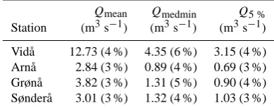
[image:13.595.329.524.389.467.2]maximum irrigation decreases by 13 % and 8 %, respectively, compared to the previously calculated values using the DBS method (Table 5). However, the effects are still significant for the minimum stream discharge where reductions of up to 20 % are observed. In extremely dry summers the effect of CO2enrichment on transpiration does not see its full poten-tial on transpiration. The low water content of the root zone limits the actual transpiration to rates below the potential and the reduction in potential ET due to increasing CO2has a rel-atively low impact on the actual flux. Hence, the reduction in transpiration because of increasing CO2concentrations is not
Table 8. Stream flow indicators for the future scenario (DBS method) with increased atmospheric CO2. Changes relative to the DBS scenario without increased CO2, Table 7, are presented in parenthesis.
Qmean Qmedmin Q5 % Station (m3s−1) (m3s−1) (m3s−1)
Vid˚a 12.73 (4 %) 4.35 (6 %) 3.15 (4 %) Arn˚a 2.84 (3 %) 0.89 (4 %) 0.69 (3 %) Grøn˚a 3.82 (3 %) 1.31 (5 %) 0.90 (4 %) Sønder˚a 3.01 (3 %) 1.32 (4 %) 1.03 (3 %)
able to neutralise the effect of climate change on irrigation and the resulting low flow.
6 Discussion
change or the uncertainty of future changes to irrigation or low flow, but rather to investigate the possible nature of the changes.
The DC method yield results on the mean behaviour of both climate and discharge which are comparable to those of the DBS method. These results corroborates with the find-ings of van Roosmalen et al. (2011). The average yearly amount of days which sees precipitation are almost similar for the two methods, however, large differences are found for the summer months where irrigation is applied. Addition-ally, the DC method does not account for the changes in the inter-annual variability projected by the climate model, as the DBS method does, which further enhances the discrep-ancy between the results obtained using the two methods. This supports the findings of Yang et al. (2010) where the DBS method was found to preserve the trends in precipita-tion identified in the raw RCM outputs. In contrast to the DC approach, the peak flow response generated by a hydrological model was found to be sensitive to the choice of RCM when DBS was used. It was found that the DC method primarily transfers the main trends of the climate model but not the an-nual variability while the DBS approach is more influenced by the variability of the selected climate model. Hence, in situations where the climate model projects variations in fu-ture climate that is significantly different from the historical climate discrepancies in resulting impacts may be expected. Most significantly in the current study, the DBS method pre-serves the large variability in the summer precipitation even though the mean summer precipitation is comparable for the two methods. Therefore, application of the DC method re-sults in underestimation of the frequency of dry summers.
When forcing the hydrological model with the adjusted climate data from the two bias-correction methods without inclusion of irrigation, two diverging trends are observed in stream flow. While a decrease in low stream flow is gener-ally predicted when using the DC method, a general increase is predicted using the DBS method. This may be counterin-tuitive, as the DBS predicts significantly drier summers than the DC. However, it illustrates the importance of base flow in low flow situations, as the increase in winter groundwater recharge in turn increases the low stream flow. In the study catchment, low flow in the streams is controlled by ground-water inflow and therefore the groundground-water level. Since the groundwater level in the catchment depends on groundwa-ter recharge during wingroundwa-ter and to a lesser extent on sum-mer climate, the differences in sumsum-mer precipitation found by the two bias-correction methods have minor effects on minimum stream discharge. However, not only the amount of recharge but also the month in which the recharge occurs is important. Spring recharge, particularly the recharge that oc-curs immediately before low flow situations may occur, has a significantly higher impact on the summer stream flow. Fig-ure 10 shows that average recharge in April is 260 % higher in the future scenario than in the current scenario when using the DBS method. The same number using the DC method
is 25 %. This explains why an increase in low stream flow is found when using the DBS method and a slight decrease is found when using the DC method. However, for catch-ments where summer stream discharge is controlled by near-surface mechanisms such as drainage flow and overland flow, the differences in variability in summer precipitation may be important.
The choice of bias correction method proved to have a pro-nounced effect on the irrigation and the resulting effects on low flow. Maximum annual irrigation is found to be almost twice as large for the DBS method as for the DC method. The abstraction of groundwater for irrigation impacts the low flow in the streams and large differences are therefore pre-dicted for both median minimum and 5-percentile flow us-ing the two bias-correction methods. Application of the DC method may result in an underestimation of the irrigation and an overestimation of low flow in the streams. Care should therefore be taken when using the DC method to evaluate aspects of the hydrological cycle that are dependent on the variability of the meteorological data.
Enrichment of the CO2content of the atmosphere and the effects on plant transpiration was found to have significant impact on stream flow. The reduced potential ET of the crops results in a lower need for irrigation. The observed increase in stream discharge due to the increase in CO2concentration corresponds to a decrease in the effects that climate changes and irrigation have on the stream flow by 50 %–65 %. The results indicate, however, that in dry periods where transpi-ration of the plants are limited by water availability the latent heat flux is not significantly affected by this mechanism. The effect of CO2on plant evapotranspiration is still highly un-certain (see e.g. Zhu et al., 2012), and more research should be done to quantify this effect more precisely. Furthermore, the increase in CO2is in this study described only by lim-iting the transpiration of the plants. CO2 also acts as plant fertilizer, and an increase in CO2could cause an increase in aboveground biomass and hence leaf area index as shown experimentally by Qiao et al. (2010), who also found that el-evated CO2 did not have any significant effect on ET. The dynamic feedback of the plants is thus not included in this study, which could be a serious limitation. Finally, the grow-ing season is likely to be extended in the future, which was not considered in this study either.
7 Conclusions
were taken into account by limiting the potential reference evapotranspiration of crops.
The DC method and the DBS method predict increases in mean annual precipitation and mean stream discharge of comparable magnitude, but there is a relative large discrep-ancy in the irrigation and low flow using the two methods. While the DC method is able to reconstruct the mean pre-cipitation and reference ET of the simulated future climate, it is not able to reconstruct the variance. This inability re-sults in large discrepancies in irrigation predicted by the two methods; partly due to differences in the predicted summer precipitation and partly due to differences in irrigation. As the variance of the DC method is controlled by the variance of the historical climate, it is not able to mimic the projec-tions of the climate model, and thus underestimates the inter-annual variability of the future climate. This underlines the fact that when evaluating objectives that are highly depen-dent on the variability of the meteorological data, such as irrigation and low stream flow, the DC method is not ade-quate. It is in those cases necessary to use a bias correction method that takes the variability of the climate model into account. The difference in variance between the two bias cor-rection methods does however not result in a clearly different low stream flow, as one might expect. This is due to the low stream flow in the studied catchment being a function primar-ily of spring recharge. The increase in late spring recharge found with the DBS method thus compensates for the drier summers and increased irrigation.
Acknowledgements. The study was funded partly by The Interreg
IVB North Sea Region Programme, European Union, for the project CLIWAT (www.cliwat.eu), and partly by a grant from the Danish Strategic Research Council for the project HYdrological Modelling for Assessing Climate Change Impacts at differeNT Scales (HYACINTS – www.hyacints.dk) under contract no: DSF-EnMi 2104-07-0008.
Edited by: G. H. P. Oude Essink
References
Abbot, M. B., Bathurst, J. C., Cunge, J. A., O’Connell, P. E., and Rasmussen, J.: And Introduction to the European Hydrological System – Systeme Hydrologique Europeen, SHE: 2. Structure of a Physically-based, Distributed Modeling System, J. Hydrol., 97, 61–77, 1986.
Allen, R. G., Pereira, L. S., Raes, D., and Smith, M.: Crop Evap-otranspiration: Guidelines for Computing Crop Water Require-ments, FAO Irrigation and Drainage paper, 56, Food and Agri-cultural Organization of the UN, Rome, ISBN 92-5-104219-5, 1998.
Allerup, P., Madsen, H., and Vejen, F.: A comprehensive model for correcting point precipitation, Nord. Hydrol., 28, 1–20, 1997. Bates, B. C., Kundzewicz, Z. W., Wu, S., and Palutikof, J. P.:
Cli-mate Change and Water. Technical Paper of the Intergovernmen-tal Panel on Climate Change, IPCC Secretariat, Geneva, 210 pp., ISBN: 978-92-9169-123-4, 2008.
Christensen, J. H., Rummukainen, M., and Lenderink, G.: Formu-lation of very-high-resolution regional climate model ensembles for Europe [Research Theme 3], ENSEMBLES: Climate Change and its Impacts: Summary of research and results from the EN-SEMBLES project, Met Office Hadley Centre, UK, 47–58 pp., 2009.
Conley, M. M., Kimball, B. A., Brooks, T. J., Pinter Jr., P. J., Hunsaker, D. J., Wall, G. W., Adams, N. R., LaMorte, R. L., Matthias, A. D., Thompson, T. L., Leavitt, S. W., Ottman, M. J., Cousins, A. B., and Triggs, J. M.: CO2enrichment increases water-use efficiency in sorghum, New Phytologist, 151, 407– 412, doi:10.1046/j.1469-8137.2001.00184.x, 2001.
DHI: MIKE SHE user manual volume 2: Reference guide, DHI Software 2011, 1–444, DHI Water and Environment, Hoersholm, Denmark, 2011.
D´ıaz, J. A. R., Weatherhead, E. K., Knox, J. W., and Gamacho, E.: Climate change impacts on irrigation water requirements in the Guadalquivir river basin in Spain, 149–159, Reg. Environ. Change, 7, 149–159, doi:10.1007/s10113-007-0035-3, 2007. Dijkstra, P., Schapendonk, A. H. M. C., Groenwold, K., Jansen, M.,
and Van de Geijn, S. C.: Seasonal changes in the response of win-ter wheat to elevated atmospheric CO2concentration grown in open-top chambers and field tracking enclosures, Global Change Biol., 5, 563–576, doi:10.1046/j.1365-2486.1999.00249.x, 1999. Doherty, J.: PEST: Model-independent Parameter Estimation. User manual, 5th Edn, 1–336, Watermark Numerical Computing, Brisbane, QLD, Australia, 2004.
D¨oll, P.: Impact of climate change and variability on irrigation re-quirements: A global perspective, Climatic change, 54, 269–293, doi:10.1023/A:1016124032231, 2002.
Ekstr¨om, M., Jones, P. D., Fowler, H. J., Lenderink, G., Buishand, T. A., and Conway, D.: Regional climate model data used within the SWURVE project – 1: projected changes in seasonal patterns and estimation of PET, Hydrol. Earth Syst. Sci., 11, 1069–1083, doi:10.5194/hess-11-1069-2007, 2007.
EUROSTAT: Water Abstracted for Agriculture, available at: epp. eurostat.ec.europa.eu (last access: 10 January 2012), 2012. FAO: AQUASTAT – FAO’s Information System on Water and
Agri-culture: Global Map Of Irrigation Areas – Denmark, available at: http://www.fao.org/nr/water/aquastat/irrigationmap/dk/index. stm (last access: 15 February 2012), 2012.
Fischer, G., Tubiello, F. N., van Velthuizen, H., and Wiber, D. A.: Climate change impact on Irrigation Water Requirements: Effects of Mitigation, 1990–2080, Technol. Forecast. Soc., 74, 1083–1107, doi:10.1016/j.techfore.2006.05.021, 2007.
Greve, M. H., Greve, M. B., Bocher, P. K., Balstrom, T., Breuning-Madsen, H., and Krogh, L.: Generating a Danish Raster-Based Topsoil Property Map combining Choropleth Maps and Point In-formation, Danish Journal of Geography, 107, 1–12, 2007. Grunzweig, J. M. and Korner, C.: Growth, water and nitrogen
Gutowski Jr., W. J., Kozak, K. A., Arritt, R. W., Christensen, J. H., Patton, J. C., and Takle, E. S.: A possible constraint on regional precipitation intensity changes under global warming, J. Hy-drometeorol., 8, 1382–1396, doi:10.1175/2007JHM817.1, 2007. Harrar, W. and Henriksen, H. J.: Groundwater model for Sneum-Bramming-Holsted ˚A Aquifer System: Set-up and Calibration, The Geological Survey of Denmark and Greenland, unpublished report, Copenhagen, Denmark, 1996.
Hay, L. E., Wilby, R. L., and Leavesley, G. H.: A Compar-ison of Delta Change and Downscaled GCM Scenarios for Three Mountaneous Basins in the United States, JAWRA J. Am. Water Resour. As., 36, 387–397, doi:10.1111/j.1752-1688.2000.tb04276.x, 2000.
Henriksen, H. J. L., Troldborg, L., Nyegaard, P., Sonnenborg, T. O., Refsgaard, J. C., and Madsen, B.: Methodology for Construction, Calibration and Validation of a National Hydrological Model for Denmark, J. Hydrol., 280, 52–71, 2003.
Intergovernmental Panel on Climate Change (IPCC): Climate Change 2007: The Physical science basis: Contribution of Work-ing Group I to the Fourth Assessment Report of the Intergovern-mental Panel on Climate Change, edited by: Solomon, S., Qin, D., Manning, M., Chen, Z., Marquis, M., Averyt, K. B., Tignor, M., and Miller, H. L., Cambridge University Press, New York, 2007a.
Intergovernmental Panel on Climate Change (IPCC): Climate Change 2007: Impacts, Adaptation, and Vulnerability: Contribu-tion of Working Group II to the Fourth Assessment Report of the Intergovernmental Panel on Climate Change, edited by: Parry, M. L., Canziani, O. F., Palutikof, J. P., van der Linden, P. J., and Hanson, C. E., Cambridge University Press, New York, 2007b. Intergovernmental Panel on Climate Change (IPCC): Data
Distri-bution Centre – Carbon Dioxide: Projected emissions and con-centrations, available at: http://www.ipcc-data.org/ddc co2.html (last access: 5 November 2011), 2011.
Jacobs, C. M. J. and DE Bruin, H. A. R.: The Sensitivity of Regional Transpiration to Land-Surface characteristics – Significance of Feedback, J. Climate, 5, 683–698, 1992.
Jones, C. G., Will´en, W., Ullerstig, A., and Hannsson, U.: The Rossby centre regional atmospheric climate model: Part I: Model climatology and Performance for the Present Climate over Eu-rope, Ambio, 33, 211–220, 2004.
Kristensen, K. J. and Jensen, S. E.: A Model for Estimating Actual Evapotranspiration from Potential Evapotranspiration, Nord. Hy-drol., 6, 170–188, 1975.
Krujit, B., Witte, J.-P. M., Witte, Jacobs, C. M. J., and Kroon, T.: Effects of rising atmospheric CO2on evapotranspiration and soil moisture: A practical approach for the Netherlands, J. Hydrol., 349, 257–267, doi:10.1016/j.jhydrol.2007.10.052, 2008. Medlyn, B. E., Badeck, F. W., De Pury, D. G. G., Barton, C. V. M.,
Broadmeadow, M., Ceulemans, R., De Angelis, P., Forstreuter, M., Jach, M. E., Kellomaki, S., Laitat, E., Marek, M., Philippot, S., Rey, A., Strassemeyer, J., Laitinen, K., Liozon, R., Portier, B., Roberntz, P., Wang, K., and Jarvis, P.G.: Effects of ele-vated CO2on photosynthesis in European forest species: a meta-analysis of model parameters, Plant Cell Environ., 22, 1475– 1495, doi:10.1046/j.1365-3040.1999.00523.x, 1999.
Piani, C., Haerter, J. O., and Coppola, E.: Statistical bias correction for daily precipitation in regional climate models over Europe, Theor. Appl. Climatol., 99, 187–192,
doi:10.1007/S00704-009-0134-9, 2010.
Qiao, Y., Zhang, H., Dong, B., Shi, C., Li, Y., Zai, H., and Lui, M.: Effects of elevated CO2 concentration on growth and water use efficiency of winter wheat under two soil water regimes, Agr. Water Manage., 97, 1742–1748, doi:10.1016/j.agwat.2010.06.007, 2010.
Scharling, M.: CLIMATEGRID-DENMARK: Precipitation 10x10 km (ver. 2), Danish Meteorological Institute, Technical Report 99–15, Danish Meteorological Institute, Copenhagen, 1999 (in Danish).
Scharling, M.: CLIMATEGRID-DENMARK: Comparison of po-tential evaporation calculated using the Makkink equation and the modified Penman Equation, Danish Meteorological Insti-tute, Technical Report 01–19, Danish Meteorological InstiInsti-tute, Copenhagen, 2001 (in Danish).
Siebert, S., Burke, J., Faures, J. M., Frenken, K., Hoogeveen, J., D¨oll, P., and Portmann, F. T.: Groundwater use for irrigation – a global inventory, Hydrol. Earth Syst. Sci., 14, 1863–1880, doi:10.5194/hess-14-1863-2010, 2010.
Sonnenborg, T. O., Christensen, B. S. B., Nyegaard, P., Hen-riksen, H. J., and Refsgaard, J. C.: Transient Modeling of Regional Groundwater Flow Using Parameter Estimates from Steady-State Automatic Calibration, J. Hydrol., 273, 188–204, doi:10.1016/S0022-1694(02)00389-X, 2003.
Stisen, S., Sonnenborg, T. O., Højbjerg, A. L., Troldborg, L., and Refsgaard, J. C.: Evaluation of Climate Input Biases and Water Balance Issues Using a Coupled Surface-SubSurface Model, Va-dose Zone J., 9, 1–17, doi:10.2136/?vzj2010.0001, 2011. Stisen, S., Højberg, A. L., Troldborg, L., Refsgaard, J. C.,
Chris-tensen, B. S. B., Olsen, M., and Henriksen, H. J.: On the impor-tance of appropriate precipitation gauge catch correction for hy-drological modelling at mid to high latitudes, Hydrol. Earth Syst. Sci., 16, 4157–4176, doi:10.5194/hess-16-4157-2012, 2012. Styczen, M., Hansen, S, Jensen, L. S., Svendsen, H., Abrahamsen,
P., Børgesen, C. D., Thirup, C., and Østergaard, H. S.: Standard-opstillinger til Daisy-modellen. Vejledning og baggrund, Version 1.2, April 2006, DHI Institut for Vand og Miljø, 62 pp., 2004 (in Danish).
van Dam, J. C., Groenendijk, P., Hendriks, R. F. A., and Koes, J. G.: Advances od modeling water flow in variably saturated soils with swap, Vadose Zone J., 7, 640–653, doi:10.2136/vzj2007.0060, 2008.
van Roosmalen, L., Sonnenborg, T. O., and Jensen, K. H.: Im-pact of Climate and Land Use Change on the Hydrology of a Large-Scale Catchment, Water Resour. Res., 45, W00A15, doi:10.1029/2007WR006760, 2009.
van Roosmalen, L., Sonnenborg, T. O., Jensen, K. H., and Christensen, J. H.: Comparison of hydrological simulations of climate change using perturbation of observations and distribution based scaling, Vadose Zone J., 10, 136–150, doi:10.2136/vzj2010.0112, 2011.
Wilks, D. S.: Statistical Methods in the Atmospheric Sciences, Aca-demic Press, 2nd Edn, ISBN 978-0127519661, 2005.
Yang, W., Andreasson, J., Graham, L. P., Olsson, J., Rosberg, J., and Wetterhall, F.: Distribution-based scaling to improve us-ability of regional climate model projections for hydrological climate change impacts studies, Hydrol. Res., 41, 211–229, doi:10.2166/nh.2010.004, 2010.