COSTANZA: A NUMERICAL CODE FOR THE STUDY OF THE REACTOR SPATIAL DYNAMICS IN TWO GROUPS EUR 2103 e

1 ° - Make any warranty or representation, express or implied, with respect to the accuracy, completeness, or usefulness of the information contained in this document, or that the use of any information, apparatll$, '.method, or process disclosed in this · document may not infringe privately owned rights ; or

EUROPEAN ATOMIC ENERGY COMMUNITY - EURATOM

COSTANZA

A NUMERICAL CODE FOR THE STUDY OF

THE REACTOR SPATIAL DYNAMICS

IN TWO GROUPS

by

E. VINCENT!, R. MONTEROSSO

(Euratom)

and

A. AGAZZI ( C. Gavazzi S.p.A. - Milan)

1964

Joint Nuclear Research Center Ispra Establishment - Italy

I.

II.

IIIi.

IV.

v.

VI.

VII.

VIII.

Preface

The power ~xcursion reactor and its simplified geometrical configuration

The physical equations and their transformation into a system of linear equations

The finite difference equations

The parts of the code and their function

Initial conditions

Dynamic calculation

Comparison between the conventional method of the kinetic equations and the direct solution of the

diffusion equations

Some examples of calculation

References

Page

'l

9

11

15

20

21

25

28

32

= radial buckling

= delayed neutrons' precursor density

C = core specific heat cal

cm3 °C

=

Dj = fast diffusion coefficient of reflector

D~ = fast diffusion coefficient of the Kth region

Dt = thermal diffusion coefficient of core

D~ = thermal diffusion coefficient of reflector

D~ = thermal diffusion coefficient of the Kth region

F = heat released by one fission (7.66 x 10- 12 cal)

K = infinite multiplication factor

Keff= effective multiplication factor

L = diffusion length

1

0 =lifetime of a thermal neutron in an infinite medium

1 =lifetime of a thermal neutron in a finite reactor

n = neutron density

Rk = Kth region

T = temperature (Kelvin)

To = temperature of the cold reactor

V = thermal neutron velocity

w = fast neutron velocity

~ =;=reciprocal of the reactor period

~ = total fraction of delayed fission neutrons

6t = time step

A = precursor decay constant (weighted average)

v = fission neutrons per fission

~c 2~r b · · f

6a, ~a= a sorption cross section o core, reflector

1

~ = thermal flux

~ = fast flux

= Fermi age of core

This report describes a numerical code for the study of the spatio-temporal dynamics of a reactor. It is written

for the reactor TESI in particular, which operates in

conditions of prompt criticality. This example was

cho-sen because the classical method of the kinetic eq.

is based on the assumption that the reactor is very near

criticality. The numerical method, based on the direct

solution of the time-dependent diffusion equation, in

condition of prompt criticality, should give more accura-te results than the classical one.

Although a very special type of reactor is studied here, this work is meant to be a preliminary work for a more general code for power reactors.

The code described in this report is only for one space dimension.

The case of two space dimensions is being studied and will be the subject of another report.

We are indebted to Mr. Foggi and Mr. Ricchena (T.C.R.) for

many informations on the core of the reactor TES! and on the point dynamics and for their valuable contribution during the discussions. We are also grateful to Mrs. Tamagnini

(CETIS) for the calculation made with the Pineto Code

and to Mr. Green and Mr. Caligiuri (CETIS) for the

This report contains the description of a numerical code written for the IBM 7090, and to be employed for the stu-dy of the spatio-temporal stu-dynamics of the reactor TESI.

This reactor is meant £or studying the destruction of a fuel element of any other reactor caused by a flash of high neutron flux. It operates in the following way:

from being critical at a very low power, it is made prompt critical. The flux rises very rapidly, and, as the reac-tor is not cooled during the transient, the temperature in the core rises accordingly. The core has a large nega-tive temperature coefficient and therefore when a certain value of the flux is reached, the reactor becomes under-critical and after a pulse of very short duration the flux decreases.

It is provided with a cooling system, which can bring the core to its initial temperature in two or three hours and prepares the condition for a new pulse. This cooling, how-ever, has no effect during the transients of a few seconds which will be studied here. The temperature rises as the integral of the flux and tends to its final maximum value.

The core of reactor TESI is a vertical cylinder of 145 cm

height made of a homogeneous mixture of fuel and

graphi-te. There is a radial reflector and also an upper and lower reflector 60 cm thick. The control rods are of two types. The first type is placed at the interface between core and radial reflector. When they are completely introdu-ced they separate the core from the reflector. The other type of rods are immersed from the top into the core.

direction with the same depth of insertion. We shall con-sider substituting these rods by an equivalent poison

which is homogeneously distributecl il'l the rodded part of

the reactor.

Since we dispose of a programme with one spatial dimension

only i.e. the z vertical dimension, we shall consider,

instead of the finite cylindrical core, a horizontal in-finite slab with a thickness equal to the height of the core and with upper and lower reflectors. In the cylinder there is a horizontal neutron leakage, which does not ta-ke place in the infinite slab; to compensate this the

ab-sorption cross section is increased by the quantity

B;

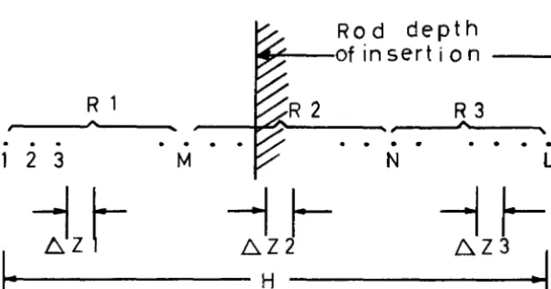
Along the z axis, see Fig. 1, we consider a mesh-points

[ZjJ

a mesh increment 6 z 1 ; in the region R 2 (core) , mesh

in-crement Az2; in the region R 3 (upper reflector) mesh

in-crement Az3. On each interface between core and reflector

is a point of the latticezM, ZN• each region must contain

at least one internal point.

The code can operate with a maximum number of 100 points.

Fig. 1.

R 1

.

.

.

2 3

1~

-jJ-.

. .

.

M

Rod depth .... ~-of insertion

R

2

.

.

.

.

.

.

N

.

.

--, r

--, r

• I

§ II rrhe physical equations and their transformation into a system_of linear equations

One of the purposes of this code is to give a description of the flux distribution in the core and reflectors and of the deformation of this distribution during the transient, due to the movement of the control rods, to the temperatu-re temperatu-reaction and to the ptemperatu-resence of temperatu-reflectors. Although in reactor dynamics it is usual to adopt the one group appro-ximation, two energy groups, fast and thermal, will be con-sidered here. With one group there is no thermal source in the reflector, whereas with two groups there is a source of thermal neutrons also in the reflector due to the

slow-ing down of the fast neutrons; this gives a much better

spatial distribution of fluxes.

There is only one group of delayed neutrons with a decay

constant A equal to the properly weighed average for the

six actual groups. This approximation is good enough

because the reactor operates as prompt critical and the delayed neutrons have an effect only on the tail of the transient.

The heat balaJ?._<;_~ equation contains only ,the term of the

heat accumulation and that of heat production, which must be equal because, as said before, no heat is removed du-ring the transient.

(II-1)

( II-2)

(II-3)

(II-4)

a

D -_faz2 - ( - + DfB )Y + k ( 1 -r.i) 1: "' + )..C

1: r ... aYJ

a

~

Dt

-2 - (

z::c

a

oz a t r ,r; v t

ac

TI

=

-

-

ll

The equations (II-1) and (II-2) are written for points in the core; in the reflectors they have the following form:

(II-5) =

(II--6)

.1

2-!E

Vat

T\.: cerm B2D which appears in the diffusion equations

in-creases the cross-sections of a quantity equivalent to the radial leakage which is not considered in this slab

geome-try. In equations (II-2) and (II-6) the term 1:p indicates

the control rod equivalent poison, which is present only

at those points of the lattice (Fig. 1 p. 4 ) which are

The fluxes '1 and </J are supposed to be zero at the outer

boundary of the reflectors (Points z₁

₌

Y(O,t) = V(H,t) = O

(II-7) (H = height of reactor)

cp (O,t)

=

=

The system of the two diffusion equations is quasi-linear because the cross section, the neutron velocities and the

quantities 't, k, c, which appear in their coefficients,

are temperature-dependent and therefore they are indirect

functionsof the flux

cp.

It is through these variable coefficients that the tempe-rature feed-back takes place.

The cross sections and the neutron velocities are calcula-ted according to

Ec ( z, t) = r, c

V

a ao T(z,t)

w(z,t) V (z,t) T(z,t)

To

where T is the uniform temperature of the cold reactor at

0 C

the initial state, and Liao , corresponding to temperature

Z:po

T •

0

v

0 are values

The quantities k, 't, c are obtained in this code by

li-near interpolation on tables given as input data.

the coefficients remain constant during this interval. This is possible only when they change very slowly with

time and for small 6t.

§ III - The finite difference e5Q_lations

The two diffusion equations can be written in the follo-wing form:

(III-1)

( III-2)

where k(k = 1, 2, 3) is the index of the region;lower

reflector, core and upper reflector respectively. The

meaning of Ak,Bk,2;E!-,P1< is evident.

The height of the reactor has been divided into mesh-points

fziJ, (i = 1,2, ••••••• L) with z₁

=

1

=

of the reactor.

On each interface between core and reflector is a point

of the lattice, and each region contains at least one

in-ternal point; t..

=

1 - Z;

=

k l l+

--region R , and can vary from region to region.

"d h .th . f h 1 .

Let us consi er t e 1 point o t e attice.

I

I

,.. •1•

A., +i

( -ii : -t, 2 ... - . L )

The coefficients Df' A, B, C, ; and Dt' E, F,

~

Let us make the integration in the space intervals

Z, 1 < Z < Z ,

1-., l and Z , < Z < Z · 1 • l

1-hj-In these intervals the coefficients are not supposed to vary.

For the sake of brevity we will carry out the calculation only for eq.(III-1); for eq.(III-2) we will give the final expressions.

z.

/ 1

.1

at

1

-( A'¥ - B</> - C)dz

2

(III-3)

z. 1

,/ 1+r

1 aY

w

at

l

dY]

_

az z.+

l

- Br/> - C)dz

z.

l

(III-4)

where

and

are respectively the left and right limit of f(z) in z =

As fluxes and neutron currents are continuous throughout the reactor it is:

[ Df ::]

z.-1

z . .

Adding (III-3) and (III-4) we obtain:

/

zi+f

1 a'l'

w

z. :I.

l - _

B <P - C) dz

2

(III-5)

The derivatives %-tare calculated with the central diffe-rences:

n n

[ J

t!

1-?I'"

. [ avJ

_{' a}

z. :I.

1-+j-=

fl.

1

The derivatives with respect to the time are approximated according to:

[!~L

1

'¥ ( z . , t ) - 'f ( z . , t

1 )

y:r:1 -

1 n 1 n- 1 1

tn - tn_

1 - - · · =

---zs-t--The integrals are approximated according to the formula:

equation (III-5) then becomes:

6.

1 fl.

2.::... + f~ 1

2 1 2

n- n-1J

'l

-v

flt .

6. 1 ₁

-- 2 _ ₊

[ n n-11

..l

'f.:n

-'11:-D 1+1 2_ +

- i+i 6.

z.

1

-'l

1'.1-'l .

J

+ D. :1. l 1-1 + A '¥n _ B </> n -C •

l • - A· 1

z.-2 l - 1

i+ 1

(III-6)

t:,.

l

If ~i is ar: ir1t('r:t:1nl point of region Rk (K = 1,2,3;

-re-= (Df li+;- = D~ and

flector; core, reflector) then

[D

l .

.Ji r

6..

1

=

=

l - l

in z. and equation (III-6) becomes:

l

D k

f y n

- -,Z i-1

ti z

k n

ti zk. B . • cp .

l. l =

' 1

t k

w.&

Ai) hk] V~

-n-1 '11 .

kl )

w . tit

(III-7)

If ~i is a_~ int on the_in~erface between Rk_

1 and Rk then

eq.(III-6) becomes:

k-1

[ k-1 Dk k-1

Df Df _k-1) 6. z

n f ₍ 1

k-1 '11. l -1 + ~1+ - - + _tizk k-1 + A. +

• tit l 2

tiz ti z w.

l

k-1 k-1 k k

n

J

k B. • tiz B . • fl z

( 1 ~ vn - _L 'Yi+1 ( l l ) cp

7!

+ + A.)

-

w~. tit l 2 i l:izk 2 2 l

r

n-1 ]

k w·i tizk

+ c. + l

-. l wf. tit 2

(III-8)

A similar result can be obtained with the integration of

equation (III-2).

The two diffusion equations of the fast and thermal groups

are then transformed into the system of 2 X (L-2) linear

equ:=:i tions:

(III-9)

- m. 'l1 ~

l1 . i - ri2't'i-1 + pi2 t. _l 2 cp. _l+ 1

=

= 2, •.•• (L-1)]

We have supposed that 'Pi

=

cft

=

1

=

=

The coefficients depend on the temperature, on the position

of the control rods and on the distribution cp~-1 and y~-1

l l

calculated at the preceding time interval.

A subroutine calculates the coefficients for every point of the lattice at every time step.

The solution of this system can be obtained with ah

iterati-ve method using alternatiiterati-vely '¥ as source of cp and cp as

source of

v,

tho-roughly described in another report ( EUR - 596e "Comparison

between the solution by an iterative and a direct method" by Monterosso and Vincenti).

The distribution \ and 'Pi are calculated at every time step by another subroutine.

The coefficients (which must be calculated at every time step according to the temperature reaction and the position of the control rods) are presumed to be constant during the interval

§ IV The parts of the code and their function

This code consists of two parts:

a) Initial condition:

this section calculates for the cold reactor:

- the uniformly distributed poison Lp for which the reactor is overcritical with a required stable period

- a critical uniformly distributed poison Lpo' or the critical depth of insertion of the control rods

-- the corresponding distribution Y(z), ~(z), C(z)

at the steady state for a required power (this power must be sufficiently small for the reactor to be con-sidered as remaining cold)

§ V - Initial conditions

Calculation of the uniformly distributed poison Lp

corresponding_t~ a desired stable period T

When the reactor is not critical, after an initial tran-sient, the flux increases exponentially according to

( ) a.t ( 1) . h .

cp t = cp

0 e , a.= T, until t e temperature reaction

takes place.

A poison ~p' as a first approximation, is introduced in

the diffusion equations; after a certain number of time

steps, the code calculates a. = ;, and corrects the value

of ~p in the sense of reducing the error ( a. -

a. ) ,

a.= 1 • The calculation is repeated until (a. - 0: ) < e:

T

where e: is an arbitrarily small quantity given as input data.

To avoid the temperature reaction, which perturbs the

sta-ble period, these calculations start from an initial

arbi-trary flux distribution at a very low power (cp C, 10

10 _{n ) ;}

cm2sec

and the reactor is considered as remaining cold during the time of this calculation.

To calculate the first approximation of Lp we use the

for-mula

a; = 1

T

=

(V-1)

even though this is valid only near criticality (in our

ca-se the reactor is prompt critical).

It is:

and

1

-'>'c

j?_

'--' + _a

- - -

---k

GO

where

substituting in (V-1) and rearranging:

z:

p

a.

V

(V-3)

(V-4)

(V-5)

Calculation of the critical uniformly distributed

poi-son ipo

With the same iterative method it is possible to

determi-" - 1

ne L,po taking

a.-:-;;-

(V-6)

It is interesting to remark that, for large values of ~,

the Ip, calculated by the code with the iterative method, is considerably different from the value obtained with for-mula (V-5); this is due to the fact that the deduction of the formulae (V-1) to (V-4) is based on simplifying

Lpo calculated with (V-6) is almost the same as the value calculated by the code with the iterative method. The small

difference is due to the inexactitude of B2 in (V-6). In

fact TESI is a reflected reactor and B2 is the buckling of

an equivalent bare reactor, the dimensions of which are de-termined by a reflector saving calculation. By substituting in (V-6) the final value of ~, it is possible to

calcula-te a more exact value of the equivalent buckling B2•

- Critical depth of insertion of the control rods

If the effect of the control rods is equivalent to a uni-formly distributed poison LpB' then it must be:

r.

-PB p L po

When the control rods are inserted the reactor is undercri-tical; when they are completely withdrawn the flux evolves

with the stable period T before the temperature reaction

takes place.

At a certain depth of insertion of the bank of control rods, the reactor is critical. To find i~ the code utilizes an i-terative method (regula falsi): at every successive position of the rods,~ is calculated and the iterations stop when

, a.f

- The distribution of fluxes at steady state

After having obtained the critical L _po , or the critical

posi-tion of the rods, the code repeats the calculaposi-tion of the

fluxes until the stable critical distribution V(z), ~(z),

The code can now reduce the fluxes to values corresponding to a desired power. This power, of course, must be suffi-ciently small to have a negligeable heat production.

The iterative calculations will be repeated a number of

ti-mes. At every iteration the thermal flux ~(z) is multiplied

by the factor

Al

core

F = --~~~~~~

£.

core

where A is the average flux in the core corresponding to

the desired power. At every iteration, the c(z) are

cal-culated according to:

C(z) =

k B L

• a _~(z)

After a number of iterations the fa.st flux 'f(z) also

rea-ches the value of steady state in equilibrium with its

§ VI - Dynamic calculation

The programme reads an initial distribution Y(z,t ); 1(z,t );

0 0

c(z,t₀) and T(z,t

0 ) at the time t0 and the control rod

posi-tion xz(t

0) . Starting from these values it calculates their

evolution in space and time according to the diffusion

equa-tions and the movement 0£ the control rods.

The calculation can start from a critical distribution obtai-ned by "Initial Conditions" at the time t

0 =

o.

possible to reinitiate, from the last distribution at the ti-me t

0 = t, an interrupted calculation.

Control rods. The movement of the control rods is simulated in a special subroutine. They can be withdrawn instantaneous-ly, or with a finite velocity which can be changed during the extraction, 0r reinsertion, according to any given law of movement.

The coefficients pi₂ of the thermal group equation are

cal-culated with or without poison for all the points of the lat-tice. The subroutine decides which points are in the rodded

or in the non rodded region and assigns to pi₂ the poisoned

or the non poisoned value.

The point zi of the non rodded region, in the vicinity of

the rod, will be partially poisoned and the total absorbtion cross-section is:

0 ~

o

where the £actor o is obtained by interpolation according

to the position 0£ the rods xz(t) between the two points

In this way the total equivalent poison in the reactor is expressed as a continuous function of the position of the rod, independently of the subdivision of the space in mesh points.

Temperature reaction. Equation (II-4) of page 6 is

trans-formed into the explicit system of L equations:

T1?

_-

r.1-

l l l _L

<p ff

= _ai

ll t c. V l

l

The~ are the unknown values of the

point z. of the lattice at the time

l

known values calculated at the time

(i= 1 2 ••••• L)

temperature at each

t · Tff- 1 are the

n' 1

( tn - tot) ; 6 . , k.,

ai 1

C. are temperature dependent and therefore they

l have

diffe-rent values from point to point, their values were

calcula-ted according to the temperature distribution Tff-1 at the

l

time ( tn - tit);

cp~

the lost calculation at time t . _n

The values of Lai' ki, Ci are therefore delayed with

re-spect to the values of

cp~.

inconsi-stency can be reduc~d by diminishing tit. Many tests were

converge to a final value for decreasing ~t. The

expe-rience has demonstrated that for ~ t ,

,o-

prac-tical improvement can be obtained (see Report EUR-596 e).

With the temperatures~ the new ~i' ci, ki are calcula-ted by interpolation between the tabulacalcula-ted values, and

the new 2'.. a ,

21> ,

for-mulae:

L, .

pi = Li _po

Vio

,ff!-1

w. = w

1 0

These values corresponding to the time tn are introduced

in the coefficients of the system (III-9) to calculate

the new distribution 0£

if1+

"':r_i.+

c:r.1+

1 1

§ VII - Cor.iparison betw~n the conventional method of the kinetic equations and the direct s_o.l.u_tiori of the diffusion equations

The conventional method for studying the dynamics of a reactor is based on the kinetics equations

( VII-1) dn

k _{eff ( 1-f3) -1} 2

+ e-B 't" _A.

C

dt = 1

.

dC k eo (3

err

~

-

(VII-2)

The following equation gives the law of the temperature va-riation

(VII-3)

_at

--

k

V L ao . n

These equations contain the space average values of n, c and T and do not consider the geometrical configuration of

the reactor. From now on we will call this the

point-me-thod. The one used in our code will be called the spatial-method.

The value of keff is determined by the control rods'

posi-tion and also by the values of k..,, -., L 2, which are knowr1

functions of the temperature. It is therefore possible to calculate the function keff(T), which, introduced ir.to e-quation (VII-1) gives the temperature reaction.

can be studied with the analogue computer, or with the di-gital code AIREC or PINETO.

However, this method is based on simplifying assumptions, which will be now explained:

a) The equations (VII-1) and (VII-2) are deduced from the one-group time-dependent diffusion equation. This deduc-tion is possible only by supposing that the flux is sepa-rable relatively to the time and space variables, i.d. the flux

<f> (r,t)

=

actually it should be:

ex,

cp ( r , t ) = n~ ₁ Rn ( r ) . Tn ( t ) (VII-5)

we consider only the first mode.

This is true only at criticality and can be assumed for states very close to criticality. The reactor TESI, how-ever, operates in conditions of prompt criticality.

b) The expressions of keff and 1 appearing in (VII-1)

contain B2 (Buckling) or the first of the proper values

of the solution (VII-5). As the reactor is reflected, B2

c) The temperature reaction given by the function keff(T) can be calculated only using a value of T averaged through-out the core. The temperature however is different from point to point and its spatial distribution changes accor-ding to the production of heat. This deforms the shape of the flux distribution and influences the reactivity. This effect can not be taken into account using this method.

d) The keff depends on the position of the control rods xz and on the temperature T. These two variables in the func-tion keff(T,xz) are non separable. However the only possible way of determining keff with the analogue computer or with the Airek Code is to consider their effect separately.

These simplifying assumptions and their consequent effects on the precision of the results can be avoided by the method of the direct solution of the time-dependent-diffusion-e-quation considered in each point of the reactor core and re-flectors.

It is interesting to compare the results of both methods for the same case. The choice of a suitable example for this com-parison is however rather difficult because the two methods have a completely different approach to the problem.

In this example, to avoid the deformation of the flux distri-bution due to the movement of the control rods, these are withdrawn instantaneously (which corresponds to a step of

reactivity in the point-method). This instantaneous

extrac-tion of the rod avoid furtherrr,ore the di£ ficul ties

explai-ned in d) ; in fact only the temperature reaction on

The control rods at the interface between core and radial

reflector are kept completely inserted. By this means it

is possible to calculate exactly the radial buckling

B;

= (

, where R

=

buckling determination (b) p. 2~ is limited to the axial

buckling.

Fixed a value of ;,the Lp can be calculated with the

i-terative method of p.~~. Then using the formulae (IV-1)

to (IV-4) it is possible to calculate the corresponding

§ VIII - Some examples of calculation

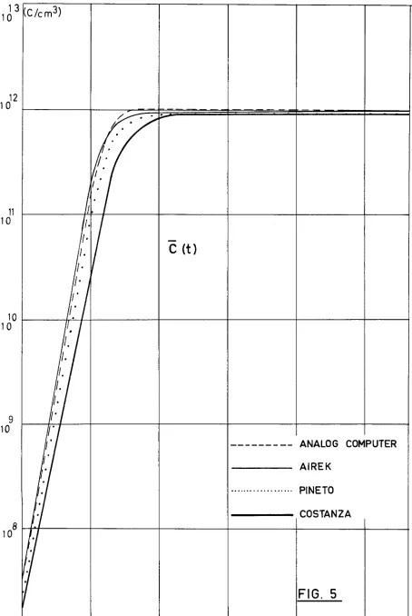
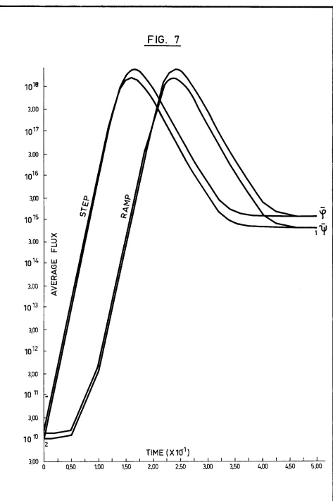
The Code Costanza can plot automatically the curves by a CALCOMP DATA-PLOTTER. See Figures 7 to 11.

a) Control rods extracted with constant veloci_!y

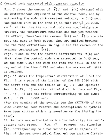
Fig. 7 shows the curves of t(t) and ~(t) obtained with

an instantaneous expulsion of the control rods, and by extracting the rods with constant velocity in 0.15 sec. The poison left in the core is,in this case,~ =0.00007

-1 . p

cm . At the time the control rods are completely

ex-tracted, the temperature reaction has not yet reached its effect, therefore the curves i(t) and ~(t) are al-most the same in both cases, they are shifted fat'wards

for the ramp extraction. In Fig. 8 are the curves of the

average temperature T(t).

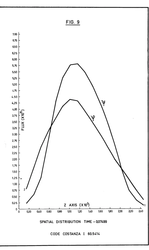
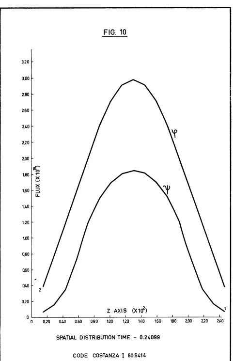
Figs. 9 and 10 are the spatial distributions V(z) and

~(z), when the control rods are extracted in 0.15 sec,

at the time 0.075 sec when the rods are still in the

co-re, and at the time 0.241 sec when the maximum of ~(t)

is reached.

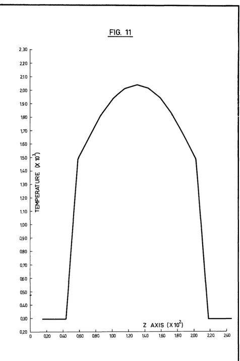
Fig. 11 shows the temperature distribution of

o.

Fig. 12 is a page of the listing of the IBM 7090 with

the input data and the tables of k , ~ and specific

oe

heat. In Fig. 13 are the initial distributions and Figs. 14, 15 , 16 are the prints corresponding to the times

o.

(For the meaning of the symbols see the WRITE-UP of the Code Costanza; some remarks and descriptions of symbols have been written with a type-writer on the listing it-self).

If the rods are extracted with a low velocity, the

oscil-lations take place. Fig. 17 reports the function

;(t) corresponding to a rod velocity of 40 cm/sec.

In

distri-bution and the control rods' positions are plotted, corresponding to the peaks of Fig. 17 at the times

t

=

=

b) Rod movements for constant power

One of the interesting operational conditions of TESI consists in reaching in a short time a certain power le-vel and in maintaining it as lons as possible, according to the temperature reaction and to the total built-in reactivity.

The desired power can be reached in the shortest time by an extremely rapid expulsion of a certain number of con-trol rods. Once the required power has been reached, the reactor must again become critical and some rods are shot into the reactor again. If in the meantime the temperatu-re has temperatu-reached a considerable level not all the extracted rods are reinserted. Some of them remain out to compensa-te the compensa-temperature reaction. Afcompensa-ter this first phase, the temperature reaction increases continuously and this will be compensated by again extracting the control rod at a reduced velocity. The total expulsion and reinsertion of

the first phase are obtained with pneumatic devices, with a maximum permissible acceleration of 100 g. The movement at reduced velocity of the second phase is obtained by

mechanical engines. An additional subroutine of the code

simulates the expulsion and reinsertion of the rods. The reduced number of rods can easily be simulated by using a convenient value of LpB in the rodded region. This sub-routine determines continuously the position of the

con-trol rods according to the power wanted and the tempera-ture reaction. The movements are kept within the limits of the maximum mechanical speed possible. Fig. 19 con-tains the curves of the rod position as function of

ti-me and of the average temperature T(t). Fig. 20

0.1 0.2 0.3 0.4

COSTANZA AIREK

ANALOG COMPUTER PINETO

FIG. 4

12

1 0

11

10

9

10

7

10

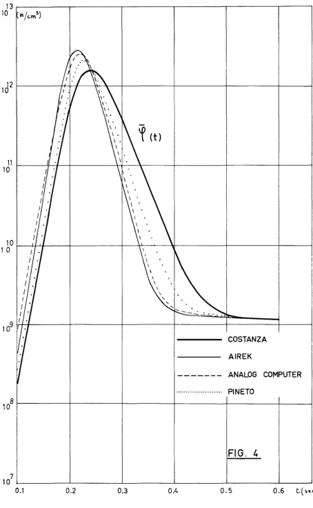
0.1 0.2 0.3

C (t)

--- ANALOG COMPUTER

AIREK

... PINETO

--- COSTANZA

FIG. 5

T

(KO)

1250

1000

750

500

293

0

•·· ,.

FIG. 7

,o18

3.00

1017

3.00

1016

3,00 Q

Lu

,_

1015 (/)

----~...;;;:::::..._ 'f'

X

--__;::::::::-.--, ii'

3.00 : )

-1

LL

1014 w

(!)

<{

a:

3.00 w _>

<{

1013

3,00

1012

3,00

10 11

..

3.00

1010 2

3.00 O _a.so

1.00 1.50 2.00 2.50 3.00 3.50 L..00 L.,50 5.00

FIG. 8

OK

19

1S

17

16

f (

15

-~

r-14 X

-

a:::

13 ::>

~

a:::

12 LLJ a.

~ _a.

LLJ Q.

I- _LU ~

11 _LLJ

....

(!) en Q:

<(

10 a::: LLJ ~

9

8

7

6

..

6.75

6.50

6.25

6.00

5.75

5.50

5.25

5.00

t..75

4.50

4.25

t..00

-0

r-0

3.75

x

3

3.00

2.75

2.50

2.25

2.00

1.75

1.50

1.25 ..

1.00

0.75

0.50

0.25 2

0 L..,__....__ _ _.__ _ ___._ _ __._ _ ___. _ _ .L--_ _.__ _ ___._ _ ___._, _ ___._ _ _ _ _ _ , . _ _ _ ~

0.20 0.40 0.60 0.80 1,00 1.20 1.40 1.60 1,80 2.00 2.20 2.L.O

0

SPATIAL DISTRIBUTION TIME - 0.07499

FIG. 10

3.20

3.00

2.80

2.60

2.40

2.20

2.00

~

1.80

....

-

LL

1.40

1.20

1.00

0.80

Q60

0.40

2

0.20

Z AXIS (X1cr)

0 ,.____...__ _ __.__ _ __._ _ __,_ _ ___. _ _ i....__...__ _ _._ _ _ _ . _ _ - - 1 . . _ - - - 1 c _ _ _ . J . . .

o 0.20 o.L.O 0.60 0.00 rno 1.20 1.t.o 1.60 1ao 2.00 2.20

u.o

SPATIAL DISTRIBUTION TIME - 0.24099

FIG. 11

2.30

2.20

2.10

2.00

1.90

1.80

1,70

1.60

M

-1.50 0

....

~

v.o

a:::

1.30 ::>

~

a:::

1.20 _a.. w

~

L!J

1.10

I-1.00

0.90

0.80

0.70

0.60

USO

0.40

ruo [

0.20

0 0.20 0.LJ) 0.60 0.80

Z AXIS (X 102)

I I I

1.00 1.20

v.o

0.14500E 02 0.14500E 02 0.14SOOE 02 0.11000E 01 0.10660E 01 0.98600E 00 0.95500E CO

OT SARZ SACZ

wz

vz

1.00000E-03 0.26350E-03 O. 24 770E-02 0.30800E 07 0.24860E 06 0.58338E-03 0.29300E 03

BU B DL SPR PREC VNU FC

0.34400E-03 0.67600E-02 0.76790E-01 0.70000E-04 1.COOOOE-04 0.24700E 01 0.76600E-11

xz TF VKP TRP TCP CSP

o. O.SOOOOE 00 -0.SSSOOE 00

o.

M = 5 N = 15 L = 19 INT = 6 Kl= 20 Kl = 0 KS = 0

T VK TAUR TAUC CS

0.29300E 83 0.18315E 01 0.42600E 03 0.40200E 03 0.25200E-00

0.39300E 3 0.18255E 01 0.42600E 03 0.39700E 03 0.35000E-00

0.49300E 03 0.18195E 01 0.42600E 03 0.3935CE 03 0.44000E-00

0.59300E 03 0.18145E 01 0.42600E 03 0.39080E 03 0.51000E CO

0.69300E 03 0.18100E 01 0.42600E 03 0.38850E 03 0.55500E 00

0.79300E 03 0.18055E 01 0.42600E 03 0.38680E 03 0.60000E CO

0.89300E 03 0.18022E 01 0.42600E 03 0.38500E 03 0.63000E 00

0.99300E 03 0.17995E 01 0.42600E 03 0.38300E 03 0.66000E 00

0.10930E 04 0.17970E 01 0.42600E 03 0.38180E 03 0.68000E 00

0.11930E 04 0.17950E 01 0.42600E 03 0.36050E 03 0.70000E 00

0.12930E 04 0.17933E 01 0.42600E 03 0.37900E 03 0.72000E 00

0.13930E 04 O. 1791 SE O 1 0.42600E 03 0.37800E 03 O. 73500E 00

0.14930E 04 0.17900E 01 0.42600E 03 0.37700E 03 0.75000E 00

0.15930E 04 0.17890E 01 0.42600E 03 0.37640E 03 0.76000E 00

0.16930E 04 0.17880E 01 0.42600E 03 0.37550E 03 O. 77000E CO

O. 17930E 04 0.17870E 01 0.42600E 03 0.37450E 03 0.78000E 00

0.18930E 04 0.17865E 01 0.42600E 03 0.37400E 03 0.78600E 00

0.19930E 04 0.17855E 01 0.42600E 03 0.37350E 03 O. 79200E 00

0.20930E 04 O. 17850E O 1 0.42600E 03 0.37300E 03 0.79ROOE 00

0.21930E 04 0.17845E 01 0.42600E 03 0.37250E 03 0.80000E 00

Fig. I2 T = temperatures

[°K]

₌

VIC=

K..,

₌

_(;m2]

CS= Specific heat of core [cal ~

o.

o.

l TR TC C PHl PH2 I\J

o. 0.29300E 03

o.

0.14500E 02 0.29300E 03 0.54178E 09 0.15561E 10 0.62595E 04

0.29000E 02 0.29300E 03 0.13901E 10 0.32396E 10 0.13031E 05

0.43500E 02 0.29300E 03 0.30251E 10 0.50483E 10 0.20307E 05

O.SBOOOE 02 0.29300E 03 0.29300E 03 0.26334E 07 0.63719E 10 0.65938E 10 0.26524E 05

g.72500E 02 0.29300E 03 0.32161E 07 0.10538E 11 0.80529E 10 0.32393E 05

.87000E 02 0.29300E 03 0.38662E 07 0.13544E 11 0.96809E 10 0.3A942E 05

0.10150E 03 0.29j00E 03 0.43997E 07 0.15676E 11 0.11016E 11 0.44312E 05

O.ll600E 03 0.29300E 03 0.47409E 07 0.16968E 11 0.11871E 11 0.47751E 05

0.13050E 03 0.29300E 03 0.48577E 07 0.17403E 11 0.12164E 11 0.48930E 05

0.14500E 03 0.29300E 03 0.471!09E 07 0.16968E 11 O.ll871E 11 0.47751E 05

0.15950E 03 0.29300E 03 0.43997E 07 0.15676E 1 1 0.11016E 11 0.44312E 05

0.17400E 03 0.29.300E 03 0.38662E 07 0.13544E 11 0.96809E 10 0.38942E 05

0.18850E 03 0.29300E 03 0.32161E 07 0.10538E 11 0.80:,29E 10 0.32393E 05

o.20

₁

0.21 SOE 0 0.29300E 03 0.30.251E 10 0.5048.3E 10 0.20307E 05

0.23200E 03 0.29300E 03 0.13901E 10 0.32396E 10 0.13031E 05

0.24650E 03 0.29300E 03 0.54178E 09 0.15561E 10 0.62595E 04

0.26100E 03 0.29300E 03 o. o. o.

VALORI MEDI 0.29300E 03 O. 399.HE 07 0.13723E 11 0.99999E 10 0.40225E 05

l TR TC C PHl PH2 N

o. 0.29300E 03 o.

o.

0.14500E 02 0.29300E 03 0.20561E 1 1 0.67748E 11 0.27252E 06

0.29000E 02 0.29300E 03 0.52886!:: 11 O. l3968E 12 0.56186E C6

0.43500E 02 0.29300E 03 0.11547E 12 0.21450E 12 0.86282E C6

0.58000E 02 0.29300E 03 0.29:;00E 03 0.27129E 07 0.24414E 12 0.27ll97E 12 0.11061E 07

O. 72500E 02 0.29300E 03 0.33090E 07 0.40034E 12 0.:-,2873E 12 0.13223E 07

0.87000E 02 0.29300E 03 0.39729E 07 0.50560E 12 0.38651E 12 0.15547E 07

0.10150E 03 0.29300E 03 0.45149E 07 0.57201E 12 0.42897E 12 0.17256E 07

0.11600E 03 0.29600E 03 0.48577E 07 O.t.Ol89E 12 0.44855E 12 0.18043E 07

0.13050E 03 0.29300E 03 0.49688E 07 0.59S95E 12 0.44259E 12 0.17803E 07

0.14500E 03 0.29300E 03 0.48400E 07 0.55595E 12 0.41112E 12 0.16537E 07 0.15950E 03 0.29300E 03 0.44823E 07 0.48585!:: 12 0.35576E 12 0.14310E 07 0.17400E 03 0.29300E 03 0.39319E 07 0.39266E 12 0. 27887E 12 0.11218E 07

0.18850E 03 0.29300E 03 0.32667E 07 0.28848E 12 0.21340E 12 0.85842E 06

0.20300E 03 0.29300E 03 0.29300E 03 0.26722E 07 0.16864E 12 Ci.16340E 12 0.65728E 06

0.21750E 03 0.29300E 03 0.79733E 11 0.11872E 12 0.47754E C6

0.23200E 03 0.29300E 03 0.36505E l 1 0.73270E 11 0.29473E 06

0.24650E 03 0.29300E 03 0.14188:: 11 0.34318E 11 0.13805E 06

0.26100E 03 0.29300E 03 o. o. o.

VALORI MEDI 0.29300E 03 0.40837E 07 0.46025E 12 0.351.37E 12 0. 141 :54E 07

Fig. I4 TO

=

ITER

=

₌

xz

=

=

VB = control rod velocity _{PHI= fast flux} ·!l

REP

=

₌

DP _{- dt} _ _d N

=

PHI _{=ltfCt) dt} Under each column are reported the

corresponding average values.

z TR TC C PHl PH2 N

o. 0.29300E 03 o. o. o.

0.14500E 02 0.29300E 03 0.63720E 17 0.37724E 18 0.15175E 13

0.29000E 02 0.29300E 03 0.16347E 18 0.77519E 18 0 •. 311B2E 13

0.43500E 02 0.29300E 03 0.35563E 18 0.11975E 19 0.48170E 13

O.SBOOOE 02 0.29300E 03 0.97205E 03 0.69883E 12 O. 74686E 18 0.16000E 19 0.43805E 13

0.72500E 02 0.10748E 04 0.83910E 12 U.12176E 19 0.20030E 19 0.42068E 13

0.87000E 02 0.11711E 04 0.97482E 12 0.15220': 19 0.23990E 19 0.48267E 13

0.10150E 03 0.12440E 04 O.lOBOCE 13 0.17190E 19 0.27141E 19 0.52984E 13

0.11600E 03 0.12b85E 04 0. 114 53 E 13 O.H3314E 19 0.29137E 19 0.55890E 13

0.13050E 03 0.13034E 04 0.11674E 13 0.186::llE 19 0.29818E 19 0.56868E 13

0.14500E 03 0.12885E 04 0.11453E 13 0.18314E 19 0.29137E 19 0.55890E 13

0.15950E 03 0.12440E 04 0.10800E 13 0.17190!:: 19 0.2:7141E 19 0.52984E 13

0.17400E 03 0.11711E 04 0.97482E 12 0.15220E 19 0.23990E 19 0.48267E 13

0.18850E 03 0.10748E 04 0.83909E 12 0.12176E 19 0.20030E 19 0.42068E 13

0.20300E 03 0.29300E 03 0.97205E 03 0.69883E 12 0.74f386E 18 0.16000E 19 0.43805E 13

0.21750E 03 0.29300E 03 0.35563E 18 O.l1975E 19 0.48170E 13

0.23200E 03 0.29300E 03 0.16:$47E 18 O. 77519E 18 0.31182E 13

0.24650E 03 0.29300E 03 0.63720E 17 0.37724E 18 0.15175E 13

0.26100E 03 0.29300E 03 o. o. o.

z TR re C PHl PH2 N

o. 0.29300E 03 o. o. o.

0.14500E 02 0.29300E 03 0.25244E 14 0.17073E 15 0.68676E C9

0.29000E 02 0.29300E 03 0.64772E 14 U.35199E 15 0.14159E 10

0.43500E 02 0.29300E 03 0.14095E 15 0.54797E 1':> 0.220421: 1 0

0.5BOOOE 02 0.29300E 03 0.14884E 04 0.14859E 13 0.296B9E 15 O. 74l17RE 15 0.17183E 10

0.72500E 02 0.16630l: 04 0.17641E 13 0.48'i22F. l'..> 0.945761:. 15 O. l "i969E 10

0.87000E 02 o. 1 snoE 04 0.20249E 13 0.60364E 1 5 0.11358E 16 0.18317E 10

0.10150E 03 0.19439E 04 0.22245E 13 0. t 8 1 25 t: 1 5 0.12ti43E 16 0.20065f: 10

0.11600E 03 0.20180E 04 0.23476E 13 0.72536E 15 O. 137F3"iE 16 0.?1130E 10

0.13050E 03 0.20428E 04 0.23f391E 13 0.7397:,E 1 5 0.14104E 16 0.?14cl6E 10

0.14500E 03 0.20180E 04 0.23476E 13 0. 72::, 3U: 1 S O. 13785E 16 0.?1130E 10

0.15950E 03 0.19439E 04 0.22245E 13 0.68125': 15 0.12848E 16 0.20065E 10

0.17400E 03 O.li:ldOE 04 0.20249E 13 0.60361,E l"> 0.1135RE 16 0.1B317E 10

0.18850E 03 O. 166.-SOl: 04 0.17641E 13 0. 48:,22E 1 S 0.94576£ 15 0.15969E 10

0.20300E 03 0.29300E 03 0.148841: 04 o. 14859f 13 0.29689E 15 o.74478£ 15 0.171f,~E 10

0.21750E 03 0.29300E 03 0.14095E 1"1 0.54797E 15 0.22042E 10

0.23200E 03 0.29300E 03 0.64772E 14 0.35199E 15 0.14159E 10

0.24650E 03 0.29300E 03 0.252•,4E 14 0. l70Bl: 15 0.68676E 09

0.26100E 03 0.29300E 03 o. u. o.

VALORI MEDI O. 18ti27E 04 0.20597E 13 O.l2u75E 15 0.116451: 16 O.lfl963E 10

1017

1016

i

101S

1014

1013

1012

0 1 2

~(t)

n

\

(\

_V

_~

V

"

~~

u

FIG.17

+.,

. : I

. r i

--1-=--r

+

-• 11;

·+ ~ +,

t__

. • . l-!

' \ f

:, ,: : :

T -1 t:±-+

-.f -±-q f r1

I+

r+.+-·I-! t

j_;I Ii '-·+i-tc+ t . •+

: :r

rtr

11\

li·'·

! ! H. I~-~ -}

L t·• ...

+

_i 1 ~ f .. :t I t

, , '.J , Jc

/1c · .

r :tl:''

. If ;1 ~+rt :i:;:::;:;±

: I ,I r

I

;::. : ff

··:: ::r +

l

:i.l ;

':H; ::: ::~ ----~ t"

;"[+ ii

l

rn ,-l-..~-b-~. :~ • 1~T

1-l: . -lf

. :J : . ····-,---,---· -

---.. :-i·

1

1+:J:1=11+1=1+1+:J:H:H=t~:tl=ll· j r f.:_J. ::r: -=-- --'"~, ·t ;_ ' 1 ~

l J

- t-.:.;" t ,-· -:

·'1\1 cc,::r,.

:';1 t1 I _.

·--·re

t ~~--~;fy~;

, I ,

1·1

ii (:

~·

'·'+:=E=.~

. :. i=.:::~ : ,

1,·

ii:

+ ' •

· ' ; '.

i1--:

tl !

~

i

V

fl

II

I'. j

ll

-J--r· Ff;_;_ ; ,...:~ l:f! _: l • t - t ,--f i I

1 '.t_: ·•-1"

Tt:

t---l-·

· · -t---~t---'--'"+-·

·_;_:_:_:_:~ -~~:+.:

.::~(-lTr.t-_-t--.-:'~. -r~

g~:

11

111 Ii

...

.... ,-...

+t ·n I r_ !

t=

•-i~ ] ( : )!ii

.c:;ir r: ·::

t; c . •+

+Hi

I~ ..

I; r .. :

· 1 « ·

·t-+-1--

'-ftt ,,

r

,re- . i

; \ttt

1-;-;r:t::"'±-c:::t-~·et~; ~ I

1 ·

·I·' '

i 1

ii

: I i 1

: j iii

• 1·1

I! I.

~~- • I • I

'1 ~

, .. :

·~· r+ 1 ll . -;-I· _{t----+-·-+"llii~}

! j

.=±=l=::1:"'-.:t:-:-ccl-H+-h-H-H-+H·H'·+rH·1; : I :

: ~~t:

f ' '] 'I !

i

, -1 ·; I i i , -,ee; 1 _{1' '}

i;

l

r

. ' i i,jj· 'i p.c,

''i .-1 t-=---1_;_

lftj. 1_~

. ' ,l

. , i

• •• 1--1-t-t +-+_:_ -~· ,r:

···1:.1:

1*tfff.Jitc;;::; :;

J'l±F tT

Jt!

1ti••

!:_;· I i ]1 .:..: t:: Ljl

~ ~ JL~tg

::~ ·:;=-cii>~-~a

'. I .

I I

1011 I I

-1010

109

10 8

10 7

FIG. 20

106

AIREK:

COHEN, E.R.:

FOX, L:

KAPLAN, S.:

P.D.Q.:

RIGHTMYER, R.D.:

SCHECHTER, S.:

STAB:

VARGA, R. S.:

WACHSPRESS, E.L.:

WANDA:

R.MONTEROSSO and

E.VINCENTI

References

"Generalized Reactor Kinetics Code"; Atomics International, No.4980.

"Some Topics in Reactor Kinetics";

Geneva Conference 1958, Volume 11,P/629 USA.

"Numerical Solution of Ordinary and Partial Differential Equations"; Pergamon Press - 1962

"Some New Methods of Flux Synthesis";

N.S.&E. 13 - 1962.

"An IBM-704 Code to Solve the Two-di-mensional Few-Group Neutron Diffusion

Equations";

WAPD-TM-70

"Difference Methods for Initial-Value Problems";

Interscience Publishers, Inc., New York.

"Quasi-Tridiagonal Matrices and Type-insensitive Difference Equations"; AEC Computing and Applied Mathematics Center - TID-4500, NY0-2542.

"A Kinetic, Three-Dimensional, One-Group Digital Computer Program";

AEEW-R.77.

"Matrix Iterative Analysis"; Prentice-Hall, Inc.

"Digital Computation of Space-Time Va-riation of Neutron Fluxes";

KAPL - 2090.

"A One-dimensional Few-Group Diffusion Equation Code for the IBM-704".

"Finite Difference Method for Solving the Spatio-Temporal Diffusion Equation in the Two-Group Approximation"

C.BONA, C.TAMAGNINI

References

PINETO - A Fortran Code for Systems of Quasi-Linear Differential Equations,

Particularly Suitable for Nuclear Reactor Dynamics.