Pipeline structure Schnorr-Euchner Sphere Decoding
Algorithm
Xinyu Mao, Jianjun Wu, Haige Xiang
State Key Laboratory of Advanced Optical Communication Systems & Networks, School of Electronics Engineering and Computer Science, Peking University, Beijing, China
Email: [email protected], [email protected], [email protected]
Received May, 2013
ABSTRACT
We propose a pipeline structure for Schnorr-Euchner sphere decoding algorithm in this article. It divides the search tree of the original algorithm into blocks and executes the search from block to block. When one block search of a signal is over, the part in the pipeline structure that processes this block search can load another signal and search. Several sig-nals can be processed at the same time in one pipeline. Blocks are arranged to lower the whole complexity in the way that the previously search blocks are the blocks those have more probability to generate the final solution. Simulation experiment results show the average process delay can drop to the range from 48.77% to 60.18% in a 4-by-4 antenna system with 16QAM modulation, or from 30.31% to 61.59% in a 4-by-4 antenna system with 64QAM modulation.
Keywords: Multiple-Input Multiple-Output System; Schnorr-Euchner Sphere Decoding; Pipeline Structure
1. Introduction
With the rapid development of wireless communications, the desire for high speed data service conflicts with the situation that fewer and fewer band width is available. Multiple-input multiple-output (MIMO), which can pro-vide dramatic high spectral efficiency, is the key tech-nology to resolve this conflict. MIMO is one of the most exciting technologies of the last decade [1,2].
The MIMO detection is rather a complex problem. The maximum likelihood (ML) detection provides the opti-mal performance. But its complexity is so high that it can not be used in actual systems. The linear detection, such as the zero forcing and minimum mean square error de-tection have low computation complexity. But their per-formance is very poor. The Vertical Bell Laboratories Layered Space Time (VBLAST) detection provides higher performance than the linear detection with the price of small complexity increase [3]. But the perform-ance is not good enough.
Sphere decoding (SD) algorithm was proposed to pro-vide optimal performance or near optimal performance with low complexity [4]. So it attracts much attention as soon as it was proposed [5]. Schnorr-Euchner SD (SESD) algorithm is an optimized SD algorithm [6]. It can find the optimal solution faster than the original SD algorithm and the modification from SD to SESD is very small. So it is the most popular optimal performance algorithm [7-15].
However, there are two main drawbacks which restrict the usage of the SESD in actual systems, especially the real time systems. One is that the calculation complexity of the SESD is not fixed and changes in a large range. Another is that it is not suitable to use in pipeline struc-ture.
In this article, we propose a pipeline structure for SESD algorithm. The searching process of SESD algo-rithm is divided into blocks and can be executed sequen-tially. When the multiple threads searching is executed simultaneously, the processing time decreases. Simula-tion experiment results show that the proposed structure can save remarkable processing time especially in low signal to noise ratio (SNR).
2. MIMO System and ML Detection
MIMO system can be depicted as an equationy = Hs + n (1)
where s is the Nt×1 transmit vector. y is the Nr×1 receive vector, and n stands for the independent and identical distributed complex zero-mean Gaussian noise. H is the Nt×Nr channel matrix where hij is the complex channel gain and satisfies Ehij2 1. Usually when
NrNt, equation (1) can be calculated. ML algorithm is to find the solution of
2
ˆML arg min
s
where means the set of all possible transmit vectors.
3. Tree Search and Euclidean Distance
For further disposition, the QR decomposition is always used to make the channel matrix triangular. We know that every matrix can be express as
H = QR (3)
equation (1) will be expressed as
ρ= Rs +η (4)
where ρ= Q yH and η= Q nH . (4) can be rewritten as
11 12 1
22 2
1 1 1
2 2 2
0
0 0
0 0 0
0 0 0
Nt
Nt
NtNt
Nr Nt Nr
r r r
r r s s r s (5)
The ML algorithm can be expressed as
2
ˆ arg min
s ρ- Rs (6)
where ˆ
ˆ1 ˆ2 ˆ
T Nt
s s s
s is the estimated value of
transmitted symbol. For sake of simplification, we set N=Nt next.
From equation (5), it can be found that there is no in-ference from other transmission signals on sN. It can be expressed as
N rNN sN N
(7) According to equation (7), sN can be calculated by
ˆ N N NN s round r
(8)
where ˆsN is the estimated transmit signal. When sN is known, sN1 can be calculated by eliminated the
inter-ference of sN. According to this idea, all transmit sig-nals can be calculated by
1
1
ˆ ˆ
N
i i ik k
k i ii
s round r s
r
(9)Equation (9) means the ith receive signal is determined by the transmit signals from the ith to the Nth one. So the solution of equation (6) can be searched from the Nth signal to the ith signal as layer by layer in a tree. That is the principle of VBLAST algorithm. Each possible transmit signal si is called a node in the searching tree. The solution finding can be depicted as searching in the tree from the root node to a certain leaf node.
VBLAST only searches the tree by one route. If there
is an error in one layer, signals in next layers will be er-ror in high probability. That is why the performance of VBLAST algorithm is not good enough. ML algorithm searches all the leaf nodes in the tree and selects the node which satisfies equation (6) from all the possible nodes. Obviously it has the optimal performance, but is a NP- hard problem.
To find the best signal as in equation (6), the distance between transmit and receive symbol should be calcu-lated. According to formula (5), the Euclidean distance (ED) can be defined as
1 2 2 1
ˆ
N N
j jk k
j k j
D r s
(10)
Also define the partial Euclidean distance (PED) as
1 2 2
ˆ
N N
i j jk k
j i k j
D r s
(11)
4. Schnorr-Euchner SD algorithm
Despite the optimal performance, the number of visited nodes of ML algorithm is the exponential function of Nt and m, where m is the signal modulation order. That is a very large number, so the complexity is too high to be utilized. SD algorithm reduces the number of visited nodes by setting a hypersphere before search and only nodes in this hypersphere will be searched. When a new leaf node is found in the hypersphere, the radius of the hypersphere is shrunk to the distance of this node. The complexity of the SD is a small fraction of that of ML.
SESD is the most important SD algorithm. It optimizes the SD algorithm by searching the smallest child node of the parent node each layer first. The first found solution is often the solution good enough. As a result, some nodes visiting can be avoided and the calculation com-plexity can be further lowered.
5. Pipeline Structure SESD Algorithm
The SESD algorithm must search the whole tree to get the solution. Each visited node must compare with the global smallest radius to determine whether or not it should be kept. Where the SESD algorithm is used, symbols should be detected one by one. Another detec-tion can only begin after one is over. As a result, the av-erage processing time can not drop easily.
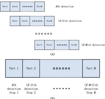
Figure 1. Pipeline structure SESD algorithm tree.
The top node of blocks is called the sub-root node of this block, from which the block search starts. Unlike the tree root node which has no practical significance, the sub-root node has its counterpart transmit signal and its PED.
There is a solution for each part, which is called the sub-solution of this part. The radius used in the SESD is still the threshold to cut node in each part. All parts share one radius although it should be updated anytime when the update condition is satisfied. The radius is called globe radius in our algorithm. Each sub-solution will update the globe radius, which will act as the cutting ra-dius in the remaining parts.
Because of the node cutting, there may be no sub-so- lution for some parts. This is not so much a bad news as a good news because that means all nodes in this part are cut and the visited nodes number in this part is often small. When a sub-solution in one part is found, the globe radius will update to the ED of this sub-solution.
Each part executes independently except one input pa-rameter and two output papa-rameters. One input papa-rameter is the cutting radius, and the output parameters are the new radius and the sub-solution of this part. So it can be processed in a pipeline structure. Each part can process at the same time. If the process of one part is over, it passes the new radius and sub-solution to the next part and be-gins a new process. There are several processes for de-coding in one pipeline at the same time. The average processing time for one detection will drop.
The structure of the proposed algorithm can be de-picted as Figure 2(a). Each detection is divided into M parts. One signal begins its step Kth detection at the time when the previous signal ends its step Kth detection and begins its step (K+1)th detection. So in a pipeline with M parts, there are M signals detection at the same time, like
Figure 2(b).
As mentioned before, if the previously processed block generates a radius small enough, most nodes in following blocks will be cut quickly. The number of vis-ited nodes will be small and the calculation complexity will be low. So we can deduce that the sequence of block
detection should be arranged in a way that the first de-tected block should be the block that will most likely generate the smallest sub-solution for the whole tree, which is the final solution. So the sequence of block de-tection should be arranged in the rising order of the PED of the sub-root, that is, just the sequence of the SESD algorithm.
6. Simulation Results
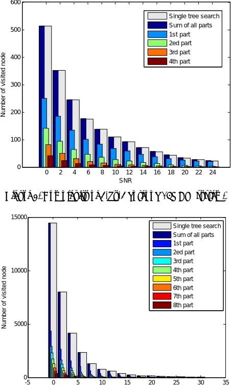
On the basis of section 5, we show the complexity of our algorithm and the SESD algorithm. The performance of the proposed algorithm is optimal as the performance of SESD, so that it is not necessary to be shown. The com-plexity is represented by the visited node number as in [16].
The complexity of the proposed algorithm is compared with the SESD algorithm in different SNRs. Also the visited node numbers of every part are listed. We convert the calculation into real field instead of complex field in both figures. But all results are the same as in complex field.
Figure 3 shows the complexity of a 4-by-4 antenna
system with 16QAM modulation. Figure 4 shows the
complexity of a 4-by-4 antenna system with 64QAM modulation.
From both figures, it can be found that the sum of the visited node number of all parts almost equals to that of the SESD algorithm, which means that the proposed al-gorithm does not increase the calculation complexity. The average process time is determined by the part that has the largest visited node number, which is the first part. Specially, in 16QAM system of Figure 3, the aver-age process time is about 48.77%, 54.34% or 60.18% of that of the SESD algorithm when SNR=0, 10 or 20dB. In
(a)
[image:3.595.313.533.509.717.2](b)
0 2 4 6 8 10 12 14 16 18 20 22 24 0
100 200 300 400 500 600
SNR
N
u
m
ber
of
v
is
it
ed node
[image:4.595.60.286.87.466.2]Single tree search Sum of all parts 1st part 2ed part 3rd part 4th part
Figure 3. Complexity of 4-by-4 antenna 16QAM system.
-5 0 5 10 15 20 25 30 35
0 5000 10000 15000
SNR
Num
b
er
o
f v
is
it
ed no
de
Single tree search Sum of all parts 1st part 2ed part 3rd part 4th part 5th part 6th part 7th part 8th part
Figure 4. Complexity of 4-by-4 antenna 64QAM system.
64QAM system of Figure 4, the average process time is about 30.31%, 52.37% or 61.59% of that of the SESD algorithm when SNR=0, 10 or 20 dB. From these data, we may find that the proportion of the visited node num-ber of the first part increases with SNR. That is because that in high SNR the probability of finding the final solu-tion in the first part is high. When the final solusolu-tion is found, most nodes in later parts will be cut quickly. As a result, the visited nodes number in later parts is small and the proportion of the first part visited node number is high. This is also indicated that the early visited part should be the part that has high probability to generate the final solution.
7. Conculsions
A novel algorithm is proposed, which divides the search tree of the SESD into blocks so that calculation can process from block to block as a pipeline structure. Sev-eral signals can be searched at the same time in one
pipe-line structure. The average processing delay drops to the range from 48.77% to 60.18% in a 4-by-4 antenna sys-tem with 16QAM modulation, or from 30.31% to 61.59% in a 4-by-4 antenna system with 64QAM modu-lation.
8. Acknowledgements
This work is supported by Nature Science Funding of China No. 61071083.
REFERENCES
[1] A. J. Paulraj, D. A. Gore, R. U. Nabar and H. Bolcskei, “An Overview of MIMO Communications - A Key to Gigabit Wireless,” Proc. Ieee, Vol. 92, No. 2, pp. 198-218, 2004.doi:10.1109/JPROC.2003.821915
[2] A. Goldsmith, S. A. Jafar, N. Jindal and S. Vishwanath, “Capacity Limits of MIMO Channels,” Selected Areas in Communicatio IEEE J., Vol. 21, No. 5, 2003, pp. 684-702. doi:10.1109/JSAC.2003.810294
[3] P. W. Wolniansky, G. J. Foschini, G. D. Golden and R. A. Valenzuela, “V-BLAST: An Architecture for Realizing very High Data Rates over the Rich-scattering Wireless Channel,” in 1998 URSI International Symposium on Signals, Systems, and Electronics. Conference Proceed-ings, Pisa, Italy, 1998, pp. 295-300.
[4] B. Hassibi and H. Vikalo, “On the Sphere-decoding Al-gorithm I. Expected Complexity,” Signal Process. IEEE Transacions, Vol. 53, No. 8, 2005, pp. 2806-2818. doi:10.1109/TSP.2005.850352
[5] C. P. Schnorr and M. Euchner, “Lattice Basis Reduction: Improved Practical Algorithms and Solving Subset Sum Problems,” Mathematical Programming, Vol. 66, No. 1-3, 1994, pp. 181-199.doi:10.1007/BF01581144
[6] K. Nikitopoulos and G. Ascheid, “Approximate MIMO Iterative Processing With Adjustable Complexity Re-quirements,” IEEE Transactions Vehicular Technology, Vol. 61, No. 2, 2012, pp. 6390-650.
doi:10.1109/TVT.2011.2179324
[7] X. Mao, S. Ren and H. Xiang, “Adjustable Reduced Met-ric-First Tree Search,” Proceedings of the 7th Interna-tional Conference on Wireless Communications, Net-working and Mobile Computing, 23-25 Sep. 2011, pp. 1-4.
[8] T. Cui, S. Han and C. Tellambura, “Probability Distribu-tion Based Nodes Pruning for Sphere Decoding,” IEEE Transactions Vehicular Technology, No. 99, 2012, p. 1. [9] J. Ahn, H.-N. Lee and K. Kim, “A Near-ML Decoding
with Improved Complexity over Wider Ranges of SNR and System Dimension in MIMO Systems,” Wireless Communications IEEE Transactions, Vol. 11, No. 1, 2012, pp. 33-37.doi:10.1109/TWC.2011.110811.110471
[11] B. Shim and I. Kang, “Sphere Decoding With a Probabil-istic Tree Pruning,” Signal Process. IEEE Transactions, Vol. 56, No. 10, 2008, pp. 4867-4878.
doi:10.1109/TSP.2008.923808
[12] X. Y. Mao, Y. X. Cheng, L. L. Ma and H. G. Xiang, “Step Reduced K-best Sphere Decoding,” Proceedings of the 76th IEEE Vehicular Technology Conference, Quebec City, Canada, 3-6, Sep. 2012, pp. 1-4.
[13] J. W. Choi, B. Shim and A. C. Singer, “Efficient Soft-Input Soft-Output Tree Detection via an Improved Path Metric,” Inf. Theory Ieee Trans., Vol. 58, No. 3, 2012, pp. 1518-1533.
doi:10.1109/TIT.2011.2177590
[14] K. J. Choi and K. S. Kim, “Hierarchical Tree Search for
Runtime-Constrained Soft-Output MIMO Detection,” IEEE Transactions Vehicular Technology, Vol. 62, No. 2, 2013, pp. 890-896.doi:10.1109/TVT.2012.2227868
[15] S.-L. Shieh, R.-D. Chiu, S.-L. Feng and P.-N. Chen, “Low-Complexity Soft-Output Sphere Decoding with Modified Repeated Tree Search Strategy,” IEEE Commu-nications Letters, Vol. 17, No. 1, 2013, pp. 51-54. doi:10.1109/LCOMM.2012.112012121728
[16] A. Schenk, R. F. H. Fischer and L. Lampe, “A Stopping Radius for the Sphere Decoder and Its Application to MSDD of DPSK,” Communications Letters, IEEE, Vol. 13, No. 7, 2009, pp. 465-467.