Parallel Algorithms for Residue Scaling and Error Correction in Residue Arithmetic

Parallel Algorithms for Residue Scaling and Error

Correction in Residue Arithmetic

Hao-Yung Lo, Ting-Wei Lin

Department of Electrical Engineering, National Tsing Hua University,Hsinchu City, Chinese Taipei. Email: [email protected]

Received August 3rd_{, 2013; revised September 11}th_{, 2013; accepted September 30}th_{, 2013}

Copyright © 2013 Hao-Yung Lo, Ting-Wei Lin. This is an open access article distributed under the Creative Commons Attribution License, which permits unrestricted use, distribution, and reproduction in any medium, provided the original work is properly cited.

ABSTRACT

In this paper, we present two new algorithms in residue number systems for scaling and error correction. The first algo-rithm is the Cyclic Property of Residue-Digit Difference (CPRDD). It is used to speed up the residue multiple error cor-rection due to its parallel processes. The second is called the Target Race Distance (TRD). It is used to speed up residue scaling. Both of these two algorithms are used without the need for Mixed Radix Conversion (MRC) or Chinese Resi-due Theorem (CRT) techniques, which are time consuming and require hardware complexity. Furthermore, the resiResi-due scaling can be performed in parallel for any combination of moduli set members without using lookup tables.

Keywords: Chinese Remainder Theorem (CRT); Error Correction; Error Detection; Parallel Residue Scaling; Residue

Number Systems (RNS); Target Race Distance (TRD); Target Residue-Digit Difference

1. Introduction

Because the residue number system (RNS) operations on each residue digit are independent and carry free prop-erty of addition between digits, they can be used in high- speed computations such as addition, subtraction and multiplication. To increase the reliability of these opera-tions, a number of redundant moduli were added to the original RNS moduli [RRNS]. This will also allow the RNS system the capability of error detection and correc-tion. The earliest works on error detection and correction were reported by several authors [1-12]. Waston and Hasting [1,2] proposed the single residue digit error cor-rection. Yau and Liu [3] suggested a modification with the table lookups using the method above. Mandelbaum [4-6] proposed correction of the AN code. Ramachan- dran [7] proposed single residue error correction. Len-kins and Altman [8-10] applied the concept of modulus projection to design an error checker. Etzel and Jenkins [11] used RRNS for error detection and correction in digital filters. In [12-16] an algorithm for scaling and a residue digital error correction based on mixed radix conversion (MRC) was proposed. Recently Katti [17] has presented a residue arithmetic error correction scheme using a moduli set with common factors, i.e. the moduli

in a RNS need not have a pairwise relative prime. In this study, we developed two new algorithms

with-out using MRD (Mixed-radix digit) or CRT (Chinese remained Theorem) for speeding-up the scaling proc-esses and simplifying the error detection and correction in RNS. The first algorithm is used for these purposes, through the residue digit difference cyclic property (CPRDD) within the range of0 x Mt1, where

r

1 2 1

t n n n

M m m _m m_{ }m_ with r additional moduli.

The moduli



m m1, 2, , mn



are called the

nonredun-dant moduli;



n1 n2 r



are the redundant

moduli. The interval,

, ,

m m _,m_n



0,M



n

1

 , is called the legitimate range, where M  _i1m_i, and the interval,



M M, 1_t



, is the illegitimate range, where

1

t r i n i

r

M MM M_m_ , and M_t is the total range. This paper is organized as follows: Section II will de-scribe the scheme the cyclic property of residue digit difference (CPRDD). Section III describes the Target Race Distance (TRD) algorithm and followed by some examples. Section IV discusses residue scaling and error correction using the TRD and CPRDD algorithms. Fi-nally, the conclusion is given in section V.

2. Error Detection and Correction Using

Residue Digit Difference Cyclic Property

Any residue digit xi representation in moduli set



1 2 n



has its cyclic length with respect to its

module number. For example, if the moduli set is (4, 5, 7, , , ,

9), then the cyclic lengths of any residue digits



x x x x1, , ,2 3 4



are 4, 5, 7 and 9, respectively. Since these

cyclic lengths are not equal, they are very difficult to use as tools for error detection and correction. Actually, there exists the property of common (uniform) cyclic length in RNS between residue digital-differences (RDD). Con-sider three moduli set



m m m1, 2, 3

 

 2, 3, 5



. The resi-

due representations and their corresponding digit-diffe- rences are shown in Table 1 and defined as the differ-

ence in value between two digits,

i

ij i j _m

d  x x , where ijs are all modulo to positive values with respect

to d

j

m if the cycle length of m_j is assigned.

Note that the residue digit-differences dij mi in

Ta-ble 1 are obtained from

i

i j _m

x x if m_i m_j , and

from

k

j k _m

x x if m_j m_k. This difference of



xixj



or



xjxk



in values may be positive or ne- gative, depending upon x_i x_j or m_j m_k and

i j

x x or x_j x_k, respectively

All negative values must be modulo to positive values. For example, on starred row 28, as shown in Table 1, the

digit difference in value for x₁0 and x₃3 is

13 0 3 3

d     . It results in d13 32 1

From the cyclic property of residue-digit difference (CPRDD) in RNS, we now have the following theorem.

Theorem 1. For a moduli set



m m1, 2, , , , mi mj, , m



n



and residue representation for x x x1, , , , , ,2  x xi j  xn



in RNS, there exists a cyclic property in differences between two residue digits,

i

ij i j _m

d  x x or

j i j _m

x x . The cyclic length can be

assigned, either to mi or mj

m

, depending upon modulo operation with respect to i or mj.

Proof: Consider the case respective to m_j, the resi-due-digit difference (RDD) between two digits in



1, , , , , ,2 i j n



X  x x _ x x _ x can be in general expressed

by the equation

i i

ij i j _m i i j j

m

d  x x  x pm  x qm (2-1)

where p0,1, ,



mj1







0,1, , _i 1 q _ m 

and i j p q, , , are integers.

For simplicity, we only consider the case of mi mj

and assume j i , and the case of can

be obtained in a similar way.

m m r m_i m_j

The related theorem and algorithm are described as follows.

1) In cycle 0, (the initial cycle), we have



0,1, , 1

j j

X x  _ m 



with q0,

0 ?

d   x x 

i i

[image:2.595.307.537.102.725.2]

ij i j _m xip mixj _mAs xj  xi p

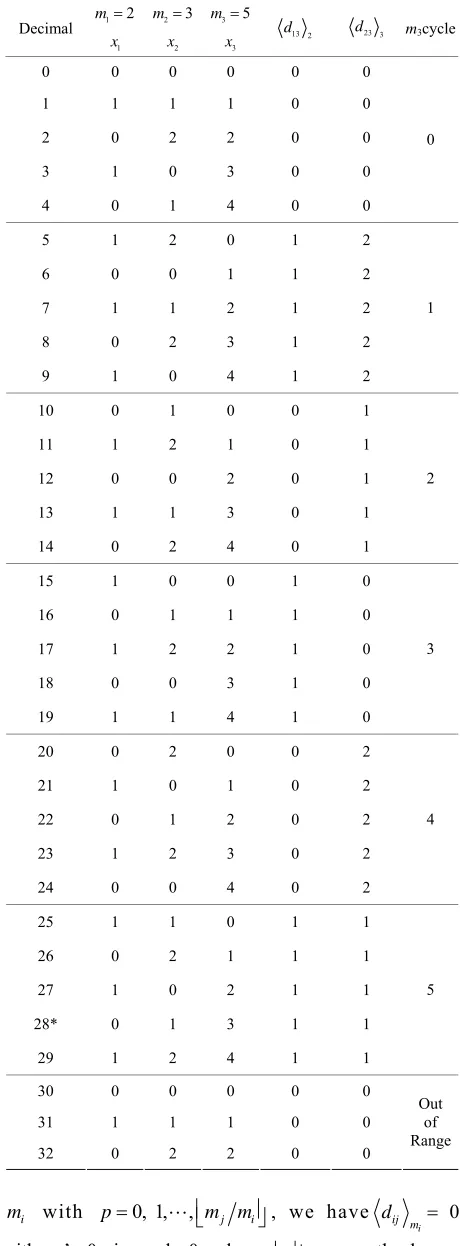
Table 1. Cyclic property of Residue Digit Difference.

Decimal m12

1

x

2 3

m 

2

x

3 5

m 

3

x d13 2 d23 3 m3cycle

0 0 0 0 0 0 1 1 1 1 0 0 2 0 2 2 0 0 3 1 0 3 0 0 4 0 1 4 0 0 0

5 1 2 0 1 2 6 0 0 1 1 2 7 1 1 2 1 2 8 0 2 3 1 2 9 1 0 4 1 2 1

10 0 1 0 0 1 11 1 2 1 0 1 12 0 0 2 0 1 13 1 1 3 0 1 14 0 2 4 0 1 2

15 1 0 0 1 0 16 0 1 1 1 0 17 1 2 2 1 0 18 0 0 3 1 0 19 1 1 4 1 0 3

20 0 2 0 0 2 21 1 0 1 0 2 22 0 1 2 0 2 23 1 2 3 0 2 24 0 0 4 0 2 4

25 1 1 0 1 1 26 0 2 1 1 1 27 1 0 2 1 1 28* 0 1 3 1 1

29 1 2 4 1 1 5

30 0 0 0 0 0 31 1 1 1 0 0 32 0 2 2 0 0 Out

of Range

i

m with p0, 1, , mj mi, we have 0 i ij _m

d 

integer less than or equal to x.

i i

ij i j _m i i j j

m

d  x x  x pm  x qm where

Thus, the RDD has mj’s “0” in the initial cycle for each modulus, i.e., in cycle 0,



0, 0, , 0



i ij _m

d  _ for

all i j.





0,1, 2, , 1 , 0,1, , 1

i i

x  _ m  _ r









0,1, 2, , 1 , , 1, , 1 1

j i i i i

x   m  m m   m   r mj

2) Next consider each modulus mi, _{For RDD = 0 (for cycles 0, , 2 , ,}

i i j i i)

m m  _m m m_

Since xiXpmi and xj X qmj,

then then



 





 















0 0 , 1 1 , , 1 1 , 0 , 1 1 , , 1 1 0, 0, , 0

i i i

i

ij m i i i m i m i m

d    _ m   m  _ m  m   m    r r 

    

with mj’s 0 s.

For RDD = 1 (not necessary in cycle 1),



 





 





1 0 , 2 1 , , 1 , 1 , 1,1, ,1

i i

ij _m i i i _{i m}

d _   _m  m  _ m  m _

   



with mj’s 1 s.

…

For RDD = mi− 1











 







 









1 0 , 1 , 1 2 , 1 , 1 , , 1

i i

ij _m i i i _m i i i

d  m   m  m    m  m  m 

  

with mj’s 1



mi



s. cyclic length is m mi j. Thus the number of cycles within

this cyclic length for N_i is _i i j _j

i

m m N

m

 

Corollary 1. From the above theorem, we can immedi- ately obtain that each cycle in the residue-digit difference of x will start at location 0, and end at location

m , and for

, i j

j j i

j

m m

m N m

m

  .



m m m_{i j k} 1



M_p 1.

Corollary 2. It is easily shown that there exists mi

number of cycles with respect to the cyclic length of Theorem 2. The algorithm of theorem 1 and its corol-laries can be extended to two or more pair-wise residue- digit differences.

p

M .

Proof. Since the residue-digit difference of



1, , , , , ,2 i j n



x x x  x x  x representation is pair-wise, the legitimate range of this pair-wise RDD



x x_i, _j



is

, (from 0 through

i j

m m m m_{i j}1). From corollary 1, the

Proof: consider a three moduli set, we have two pair- wise moduli sets, whose RDD (Residue Digital Differ-ence) is

j k k

k _k j

k

jk m m m _m j j m k k m

m

d  X  X  x qm  x sm

Assume mk mj r₂, and also pair-wise numbers



 

where mk is again the referenced module.





2

0,1, 2, 1 , 0,1, , 1

j j mj r



Follow the same procedure as step (2) as above. x  _, m 2 ,  _  and



 





 

2







0,1, 2, , 2 , 1 , , 1 , , 1 1

k j j j j j

x  _ m  m  m m  _ m  r   m_k .

1) For q s 0,x_j x_k, 0x x_j, _k m_k1,d_jk 0 thus

0,0, ,0, , , , ,

j j j mj

jk _m j _m j _m j

d __ m m  m



’s j

m “0” r2’s “ –

j j _m

m ”

 

0

This shows that j jk _m

d has also “0”s in cycle 0

of

k m



0, 1, 2, , 1



k k k

m x  _ m  . The cyclic length is

 

mj 

 

mk  r2, and the number of cycles for mj is



2 ormjmk mj



k mj r mjmk mj

0

q s

m .

j jk _m

d 

 

2) For and h (a constant for any

RDD), if xj xk



 















’ “ ”

0 , 1 1 , , 0 , 1 1 ,

j

j j

k

jk _m j m j

m

m s h

d  h h  _   m h    m  h _



for mj is still mk



mjmk mj



. Combining these

three moduli



m m m_i, _j, _k



into one set, we have cyclic This shows that the

j

jk _m

d h in any location has

length Mp m mi jmk (for example,

1 2 3 2 3 5 30

m m m      ). The number of cycles for

1, 2, 3

m m m are ,

1 2 3 3 5 15

m

N m m   

2 1 3

2 5 10N_m m m    , and ,

respectively. As shown in Table 1, the RDD pairs of

3 1 2 2 3 6

m

N m m   





         

 3 3

13 2 23 3

All 5 pairs in each cycle.

, are 0, 0 , 1, 2 , 0,1 , 1, 0 , 0, 2

m m

d d



, and

(1, 1)

In general, M_p m m₁ ₂ _ m_k _ m_n and

k

m p

N M m_k with m_k rows and



n1 RDD



in each row.

This completes the proof. Example 2-1.

Consider a moduli set



m m m1, 2, 3

 

 4,5,7



, X 9

and its corresponding residue digits representation set is



1, 4, 2



. The cyclic length is 140



  4 5 7



2

m m m

20 N

and the number of cycles for 1 , and 3 are

, and ,

1 35, 2 28 m3

m m

N  N   , respectively. Error detection and correction:

Before the CPRDD algorithm used for error detection and correction is described, some basic terms in use must be defined.

Definition 1: Stride distance ij: It is the incremental

or decremental distance between moduli i and S

m m_j in absolute value from ith cycle to



i1 th



cycle.

For example: S23  5 7 2



. (1) Error detection

Let the moduli set be



m m, , ,_ m m_k, _k, ,_ m_{k r} ,

’s ij

d

L d



m m1, 2, , mk , ,m

 

1 2 1 where

are the nonredundant moduli and k 1 k r are the redundant moduli. Since the cyclic lengths of CPRDD are constant, it is thus easily found that the number of cycles on track ij from the starting point 0 (or other

ij) to its target position. In turn the distance of RDD’s

can also be found.

m _

Theorem 3. The number of cycles on track ij

(col-umn ij) from any starting point (say ) to its target

position can be found using the equation below; L

d dˆ_ij

ij

d

ˆ

i

ij ij ij ij

m

d S k d

where ij the stride distance between moduli mi and j and k = the number of cycles passing through

from starting point to the destination, ij

S  m

ˆ ij

d d  on

track ij If , then the number of cycles are equal

to the total cycles from the starting point “0” to its target position .

L

d

ˆ ₀

ij d 

k

ij

Proof: Since ij is the number of cycles from 0 to

ij with respect to module j, and j is the cyclic

length, thus ij j is the total distance from the starting

point ij to its target position . The remaining distance for on track in the

d m

ij

m

ij



k m

ˆ d 0

ij

d

d

L k_ij



th cycle must

be on the same row of dij on track Lij. Thus,

 

  



RDD xi RDD xj  kijmjdij , ,

.

Once the RDD’s of x x1 2 , ,x xn r are found, the error detection and correction for moduli can be found just by comparing the calculated cycles or RDD with the original residue representation, pair-wise so that the error module can be detected.

The procedure for error detection by using CPRDD algorithm is summarized as follows.

1) Choose two most significant (largest) moduli as the referred moduli among the n moduli, say mn1 and mn.

2) Find the skip distance of a cycle

n1 n n1 n S _  m_ m .

3) Find the digit difference

 1  1



1 2



dn n  xn xn mn from X  x x, , , xn1,xn . 4) Create the equation of



1





1



RDD xn,xn  d xn ,xn n m

 or



1



 1   1 



x1,



RDD ,

n n

n n n n n n n n _m

m

x x  S _ k _  d x (2-2) 5) Solve for k_{n1 n} from Equation (2-2) as the

n1 n

S _ and



₁,



? n

n n _m

d x_ x are known. The value of must be less than or equal to

n1 n k _



m m1 2  mk  mn2



.

6) Find the corresponding RDD



xn1,xn



distance

from the starting point to xn1.

7) Calculate , ,



x x1 2 ,xn



from RDD1, RDD2, ,

and check the values of



x x1, , ,2  xn

 

1, x x1, ,2 ,xn



2,

and …. If these sets’ numbers are equal, then no error occurs; otherwise, error exists.

We take the similar numerical as example 2-1 to verify this algorithm. (CPRDD)

Example 2-2. Assume that a moduli set



m m m m1, 2, 3, 4

 

 4,5, 7,9



and number X whose

resi-due representation is



x x1, 2, ,x x3 4

 

 1, 2, 6, 7

  

 97 10.

If an error occurs at m X2, 



1,3, 6, 7



, the error

detec-tion can be described as follows. Let us begin our procedures from the



3 4





3 4



RDD x x, d x x, . Since





34 3 4

13 4

23 5

le 7 9 2,

5 3,

3 2

S m m

d

d

    

  

  

skip distance of a cyc

and

34 6 79 19 8

d      . Then

 

34 34 34 9 2 34 9

N d  S k  k 8. Solve for , and let

34

k





34 1 2 20

k  m m  within legitimate range

The corresponding RDD



x x3, 4



primary distances

for these two k34 are, respectively,

 

 

1

2

RDD 4 4 7 6 34

RDD 13 13 7 6 97

   

   

Thus, the generated results of the residue representa-tion from RDD 4₁

 

and RDD 13₂

 

are respectively

  

 



1 34 1, , ,2 3 4 2, 4, 6, 7

X  x x x x  ,

  

 



2 97 1, , ,2 3 4 1, 2, 6, 7

X  x x x x  .

Since the calculated results of X1 and X2 are not

iden-tical, there must be errors in one of these moduli. We cannot determine which one is erroneous. To locate the module where the error exists, at least one additional (redundant) module must be used.

The procedure for error correction by using CPRDD algorithm is essential the same as the error detection. However, two additional redundant moduli

1

r and

2

r must be added for one error correction. Note that

only one redundant modulus added for error detection. m m

1) Choose mr₁



or mr2



as a referred modulus.

2

r

2

r

2

r 2) Find k_{     1 r1} ,k_{2 r2} , ,_ k_{  r1} as the same proce- dures of error detection steps 2-7.

3) Examine the values of . If common value exists among, ,

     1 r1 , 2 r2 , ,   r1

k k _ k

     1 r1 , 2 r2 , ,  

k k _ k _

1

r then no error occurs. If there is one and only one, say

  i r1 that has no common value with all other   1

k _{j r} ,

then an error exits in modulus . This completes the error correction procedures.

k i

m

The following example is illustrated here to verify this algorithm.

Example 2-3. Error correction

As before we can further locate and correct a single error by adding two redundant moduli,

1 and .

Let us use the same example. The moduli set r m

2

r

m



m m m m m1, 2, 3, 4, 5

 

 4,5, 7,9,11



1 9

r

m 

, where and 5

are redundant moduli and , and the residue X representation,

4

m 11 

m

2

r

m



x x x x x1, , , ,2 3 4 5

 

 1, 2, 6, 7,9

  

 9710 3

m

. If a single error occurs at , e.g. X 



1, 2,5, 7,9



, and m4 is as-

signed as a reference module, then d_{14 4}  6 ₄ 2,

24 5 55 0

d    , ₃₄

7

2

d   5,and

45 11 211

d   9. From CPRDD algorithm, we can find the number of cycles for these RDD’s.

14 14 4 5 14 4 2

S k  k  ,

24 24 5 4 24 5 0

S k  k  ,

34 34 7 2 34 7 5

S k  k  ,

45 45 11 2 45 11 9

S k  k 

Since the cycle length is 9, all above kij values must

be less than 140 16 9

 _{ }

 

  . Thus we have

14 2,6,10,14

k 

24 0,5,10,15

k 

34 6,13

k  .

45 10

k 

If no errors occur, all kij’s are equal, i.e.,

14 24 34 45

k k k k .

Compared to the above results with pairwise moduli, only k14 k24k45 10

k

meets this condition. There exists no such value in 34.

This shows that the module 3 is faulty, therefore

we can correct it as follows: since , the

m

10 14 24 45 10 k k k 

9 7 97 x

14 4

RDDk cycle length     . Thus x1 97 4 1, x2 97 52, x3 977 6,

4 979 7

x   .

This completes the error correction.

Note that the above CPRDD’s for each residue-digit difference, ij, and ij can be processed in parallel. In

addition, if the referenced module is assigned to the er-roneous module by chance, e.g., 3 this algorithm will

fail to locate the error. In this case, there are no values that can be found to match this condition. The way to solve the problem is, of course, to assign any other moduli, e.g., or m .

d k

m

m

’ ij

k s

1 2

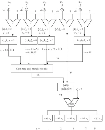
The hardware design for the proposed algorithm in Example 2-3 is shown in Figure 1.

3. The Target Race Distance (TRD) Scheme

The conversion or decoding technique from residue rep-resentation to X in binary is usually accomplished using

the mixed-radix digit (MRD) or Chinese remained theo-rem (CRT). An optimal matched and parallel converter of this kind can be seen in [13]. The MRD is shown by the following expression with weighted numbers:





1 0 2 1 3 1 2 1 2 1

0 1 1 0

1

with 1,

p

n n M

n

i i

i

x a m a m a m m a m m m

m m m m





 

    







 



where Mp m m1 2mn ni1mi, and i



0,mi1



is

the mixed-radix conversion (MRC) of x.

Optimization can be obtained using this method, as the accessed table lookup time is exactly equal to the right addition time, after immediate column stage for the tree

- - - -

-m1 m2 m3 m4 m5

1 2 5 7 9

4 5 7 9 11

x'1 x

'

2 _x'

5 x'4

x'3

7 7

25 P2 0 '₅

24 

d

2 4 14 

d

5 14 

s s24 4 s34 2 5 7

34 



d d44 90

2 '45

s

9 11

45 



d

14 , 10 , 6 , 2 14

k

2 4 14

14k 

s s24k2450 s34k34 7 5 s24k24 52

Compare and match circuits

10*9 multiplier

adder

7 4 

x

4 97

 975 977 979 9711

x = 1 2 6 7 9 10 45

k

15 , 10 , 5 , 0

5 * 0 24 



 q

k

7 7

9

11 45

45k 

s

13 , 6 7 * 6

34 r 

k

10

9 10

7 7

[image:6.595.133.472.86.505.2]

90

Figure 1. The hardware implementation for the proposed error and correction location algorithm can be accomplished with-out using lookup tables.

However, time is still consumed reading a large num-ber of lookup tables. Additional hardware complexity is required by the adder-tree networks. An algorithm called the target race distance was with a simpler structure was developed for high-speed conversion.

TRD algorithm

Suppose each residue number in the RNS i m has its own track i, and the distance over track from 0 (starting point) to i

i

i L

X

L

X (end point) through cycles can be expressed using i

k





, 0,1, , 1 ,

i i i i i i

D x k m k  _ m  .

Obviously, the primary (no multiples of mi) distance of

i

x is _min . To obtain the X from its

residue representation of

 





0

i i i

D x k 

1, , ,2 r x x _

r

x , we must find a target such thatx x₁, , ,_2 x traversing the same

dis-tances over tracks 1 2 respectively, i.e. when the

TRD distance of each target i , , , r l l _l

x is reached, then

1 2 r.

D  D _D The TRD distance of X can be found

from the following theorem:

Theorem 4. Consider the simple case of two moduli sets



m m1, 2



. Its residue representation and targets are x1 and x2 respectively. Let

 

D1 p be the primary dis-tance of residue x1 from 0 to x1 on the track L1, and

 

D2

L p

be the primary distance of x2 from 0 to x2 on track 2. Then the TRD distance for these two residues x1 and x2 that have the same TRD distances can be obtained by

the following equation.



1 2

 

 



TRD x x,  x₁ k₁ m₁  x₂k₂m₂ (3-1) In addition, k1 can be calculated from the equation

 

2 p

2

1 1 1 m 2

where m1 is the cyclic length of x1, and k1 is number of

cycles, all of the integers,

1 0,1, 2, , 2 1

k  _ m  .

Proof: It is easy to show that the above TRD



xi, xi1



is the common target distance of x1 and x2, Since

1

1 1 1 m 1

x k m x

And

2 2

2 2 2 m 2 1 1 1 m

x k m x  x k m X,

thus









2

1 2 1 1 1 1 1 1

TRD x x,  x k m _m  x k m X is the TRD distances for both of x1 and x2.

Corollary: It is evident that the above theorem can be extended to n moduli set



m m₁, ₂, ,_ m_n



and residue number



x x₁, , ,_{2 } x_n



. The corresponding TRD of



x x1, , ,2  xn



are therefore



 

 











1 2 1 1 1 2 2 1 2

3 3 1 2 3

1 1 1 2 1

TRD , , , _n

n n n

x x x x k m x k m m x k m m m

x_ k _m m m_

   

 

 



 

In addition, kican be solved from the following equa-tions.

2

1 1 1 m 2

x  k m x …

1

1 2 1

i

i i i m i

x k m m m x

 

  _ 

where k_i 0,1, ,_



m_i11



, , ,

Note that x x1 2  xn are the targets of moduli

1, 2, , n respectively and the

m m _ m TRD



x x₁, , ,_{2 } x_n



is the distance that has equal track lengths, i.e.

1 2 n

L L _L L. That is;

1 1, 2 2, 3 3, , n n

m m m m

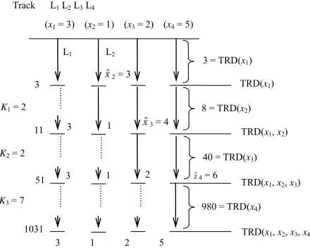
L x L x L x _ L x . Example 3-1 Let the moduli set be



m m m m1, 2, 3, 4

 

 4, 5, 7, 9



and the residue

represen-tation be



x x x x1, , ,2 3 4

 

 3, 1, 2, 5



. The procedures to

find the TRD distance can be described as follows:

1) Find the primary distance

 

D1 of residue

 

2

1 1 p 3m

x  D  since m2m1 and 3 k1 4 51

is required , thus k12, and



1 2

 



TRD x x,  3 2 4  11

2) Repeat the procedure 1 to find the number of cycles

k2 and k3 and the last TRD distances (destinations),



1 2 3



TRD x x x, , and TRD



x x x x₁, , ,_{2 3 4}



. Since xˆ₃ 11₇4

3 2 7

ˆ 4 5 2

x   k 

2 7

4  k 4 5 2

2 2

k

 

thus TRD

 

x₃    2 4 5 40 and TRD



x x x_{1 2 3}



11 40 51 

4 9

ˆ 51 6

x  

3 9

6   k 4 5 7 5

3 7

k  

thus TRD

 

x4     7 4 5 7 980

and TRD



x x x x_{1 2 3 4}



51 140 7 1031  

The final TRD distance is the common distinction of this system for targets x x x1, ,2 3 and x4 i.e.



1 2 3 4



TRD x x x x 1031X. This result can be verified as follows:

4

[image:7.595.187.407.544.720.2]

1031 3, 1031₅1, 1031₇2 and 1031₉5

Figure 2 Shows the TRD’s on tracks and

respectively. 1 2 3

, ,

l l l l₄

Error detection and correction by TRD algorithm A redundant residue number system with r1 re-dundant moduli will allow detection of any single error [4,14]. Consider the moduli set



m m m m1, 2, 3, 4

 

 4,5, 7,9



and the correct residue re-

presentation X x x x



1, , ,2 3 x4

 

 1, 2, 6, 7



97. Let us

Track L1 L2 L3L4

(x1 = 3) (x2 = 1) (x3 = 2) (x4 = 5)

3 = TRD(x1)

8 = TRD(x2)

40 = TRD(x3)

980 = TRD(x4) TRD(x1)

TRD(x1, x2)

TRD(x1, x2, x3)

TRD(x1, x2, x3, x4) 3

11

51

1031

K1 = 2

K2 = 2

K3 = 7

3 1 2 5

...

...

...

...

.

...

...

.

...

....

.. ...

....

....

.

L1 L2

3 1

3 1 2 4 = 6

3 = 4 2 = 3

assume that is the redundant moduli with a sin-gle error 4

9 m 



1, ,

 



F

X x x_{2 3 4} residue represen- tation. The TRD theorem can be used to detect this error. We find that final TRD for 1 2 3

, 1,3, 6, 7 x x 

, ,

x x x and x₄ does not fall into the legitimate range as follows i.e.



4 5 7



140 F

R    

























1 1

2 2 1

1 2 1 2

3 7 3

3 3

4 9

3 9

3

4 4

TRD 1 1

TRD 3 12 3

TRD TRD TRD 13

ˆ 13 6

TRD 6 0

ˆ 13 4

4 140 7

6

TRD 7 6 140 840.

x

x k

x x

x x

x x

k k

x  

  

  

  

 

 

  



    

The final TRD distance



1 2 3 4



TRD x x x x, , , 13 840 853 140   . If we need to locate and correct this module error, another redundant module must be added. Let us assume that m511 for

this requirement in the above residue representation. The current redundant moduli set is



m m m m m1, 2, 3, 4, 5

 

 4, 5, 7, 9, 11



and the correct

resi-due representation is



1, , , ,2 3 4 5

 

1, 2, 6, 7, 9

  

97

x x x x x x  9

m  m₅11

 . Let us as-sume that 4 and are the redundant mo-

duli. With a single error



1, , , ,2 3 4 5

 

1,3, 6, 7,9



F

x  x x x x x 



. The TRD theorem can again be used to locate and correct this error. We find that final TRD’s for x x x x1, , ,2 4

 





5 dose

not fall in the legitimate range, but other final TRD’s for 1,3, 7,9 

 



1, , ,2 3 4 1,6,7,9

x x x x  do, falls in the legitimate range:

1) TRD for x x x1, ,2 4 and x5



















1 1

2 1 2

4 1 2 4

5 11

4 11 5 4

5 1 2 4 5

TRD 1 1

TRD , 13

TRD , , 133

ˆ 133 1

1 180 9 , 2

, , , 133 360

493 140 out of legitimate range .

x

x x

x x x

x

k x k

TRD x x x x

  



 

    

 

 



2) TRD for x x x1, ,3 4 and x5









1 1

3 3 2

4 9

TRD 1 1

TRD 6 12; 3

ˆ 13 4

x

x k

x

 

  

 













3 9 3

4 1 3 4

5 11 5

5 1 3 4 5

4 28 7, 3

TRD , , 13 84 97

ˆ 97 9

, , ,

97 140 within legitimate range .

k k

x x x

x x

TRD x x x x

   

  

  



 

Thus, the error is located at module m2 and must be

corrected to x2 97 52.This algorithm can also be

used for multiple error corrections. However, at least three redundant moduli are required. The procedures are similar.

4. Scaling with Error Correction

The above proposed algorithm used for error detection and correction has the advantage of not requiring lookup tables. No CRT (Chinese residue theorem) decoding pro- cesses are required. However, it is still time consuming and requires extensive hardware complexity for each module having multiple-value inputs to the match unit and selecting a correct one as a output. To improve this drawback, an optimal matching algorithm is proposed here for the error correction. The following two theorems will be used and an example follows.

Theorem 5. Let m1 and m2 be two relative prime

num-bers in RNS for module 1 and module 2 respectively. Then there must exist the relation represented by the equation

2 1

1 1 m 2 2 m

m x  m x  k , where

2 1

1 1 2 2 2 1

0 m x _m m , 0 m x _m m so

that 0 k m2, assuming m2m1. The x x1, 2 and k

are restricted to integers.

Proof: As a first step, let . It is easily seen that

2

0 k

1

x m and x2m1 will be satisfied. Next consider

0

k . Since there are two different pair combination

2

1 1 m 2

m x m and

1

2 2 m 1

m x m, thus the difference

between m x1 1 and m x2 2 of k will always be satisfied

for 0 k m₂, where k is restricted in integers.

Theorem 6. If the values of m1 and m2 and k in the

equation

2 1

1 1 m 2 2 m are known, then p1

m p  m p  k

and p2 can always be determined from equation





1

2 1 1 _m

m m p k or





2

2 1 2 _m

m m p k, where p1,

p2 and k are within the range: 0 p1k 



m1 or m2



Proof: Let the difference value of m₂m₁ be equal to d, then d will be the integers within the range between

0 and m2, i.e., p₁0,1, 2, ,_



m₁1



, or





2

0,1, 2, ,p  _ m₂1 . These two expressions show that we can always select an integer value p, within the inter- val between 0 and



m₁1



or



m₂1



to satisfy the

conditions

1 1 m

dp k or

2 2 m

dp k

Example 4-1 Let 1 , and 2 . Find the mi-

nimum values of p1 and p2 respectively from the

follow-ing equation :

m 5

3 7

m 

1 2

7p  5p 

Since m15 and , we have

m 

2 7

m 

2



2 1 7 5

dm   ,

and

1 5

2p 3 (4-1),

or

2 7

2p 3 (4-2),

from Equation (4-1)

1 5

2p 3 so p1 4, 2 4



  



5 3,

from Equation (4-2)

2 7

2p 3, so p2 5 for 2 5



  



7 3.

This result can be verified by substituting

7 4 5 5 3    into the above equation. Theorem 6 is very useful as shown in the following example.

In Theorem 3 of Section III, the number of cycles on track from the starting point “0” to its target posi-tion “ ” can be expressed by setting , i.e.

ij

L

ij

d dˆ_ij 0

, or i

ij ij _m ij ij ij i i ij

i m

s k d s k p m d (4-3),

where sij is the module i stride distance referring to

module j. Similarly, the number of cycles on track jk

from the starting point ”0” to its target position “ l k

x ” can

be expressed by setting dˆij 0, i.e.;

2 or j

jk jk _m jk jk jk k j _m jk

s k d s k p m d (4-4)

Since, from theorem 3, the cyclic length of the residue digits differences reference to module mj is constant

(uniform), then there must exist a condition,

ij ij ij jk jk jk Eliminating the above terms

from Equations (4-3) and (4-4), c  s k c s k

ij i i jk jk k ij ij jk jk ik

c  p m c p m c d c d D

i i i k ik

p m p m  D

wherepi c pij i, pk c pjk k

d

 and

ik ij ij jk

Example 4-2 jk 

D c d c

Let the moduli set



m m m m m1, 2, 3, 4, 5

 

 4,5, 7,9,11







1, , , ,2 3 4 5





x x x x x x



1, , , ,2 3 4 5

 

 1, 2, 6, 7,91, 2,5, 7,9



, and the error

x x x x x x      , the error occurs at m3.

Follow the same procedures of the Example 4-1 to use this algorithm.

14 14 4 5 14 4 2, or 5 14 4 1 4

S k  k  k  p

24 24 5 4 24 5 0, or 4 24 5 2 5

S k  k  k  p 0 (4-6)

34 34 7 2 34 7 5, or 2 34 7 3 7

S k  k  k  p 5 (4-7)

45 45 11 2 45 11 9, or 2 45 11 5 11

S k  k  k  p 9 (4-8) Eliminating and from Equation’s (4-5) and (4-6) 14

5k 4k24

1 2

16p 25 8p 

13, and

p p

,

1 28,

solve for k14 from (4-5),

14 4

5 4 13 k   2,



k1410,

or 4k24  5 8 40,



k24 10,.

Check from Equation (4-5),

11

2 10 9, 2 10 ₇ 6 5.

This shows that the error occurs at module m3. From

this result, we can immediately obtain 2 10 ₇6. Noting that it may happen that the assigned referenced memory moduli falls coincidentally with error memory module m3. In this occurrence, we cannot find the correct

(integers) values of P1 and P2 within the legitimate range.

It seems that this algorithm can only detect error. To complete the error correction procedure, we can simply change the referenced module to any other and follow the same procedure as before. This guarantees that the pro-posed algorithm in Theorem 4 will also work well in this case. The hardware structure for illustrating this algo-rithm is shown in Figure 3.

The proposed TRD (target Race Distance) scheme used for error correction can be used for scaling and as-signing numbers in a residue number system. A redun-dant residue number system (RRNS) is defined as before in an RNS with r additional moduli. The moduli



m m1, 2, , mi, , mk



, are called the nonredundant mo-

duli, while the extra r moduli,



mk₁,mk₂, , mk r



are

the redundant moduli. The interval,



0, 1Mk



, is

called the legitimate range where k₁

k i i

M 



_m and the

interval,



M_k, 1M_kr



, is the illegitimate range, where

1

r

kr k r k i k i

M M M M



 m is the total range. In the

RRNS, the negative numbers within the dynamic range are represented as states at the upper extreme of the total range, which is part of the illegitimate range. The posi-

tive members are mapped to the interval 0,



1



2 k

M

  

 

 ,

if Mk is odd, or 0,

2 k

M

 

 

 , if Mk is even. The negative umbers are mapped to the interval

2

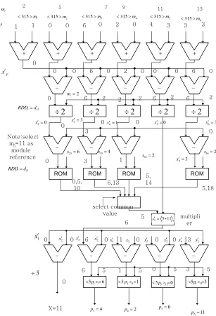
[image:9.595.302.541.90.299.2]

-ROM

10*9+7

-

-

-

-

-

-1 2 5 7 9

4 5 7 9 11

x

1'

x

'

2

x

_x

'₅

' 4

x

'3

4

10

5 410₅ 210₇ 210₁₁

7 7

16P1 25P2 0 '24₅ d

0 0 1 0

X=97

9 4

m

7

4

X 10 10 10 10

2

14

d d14'2 d240 d24'0 d346 d34'5 d459 d45'9

2

4 14 

d s14 5

2

34



s

4

24



s d34 75

0

7 44 



d

0 '44

s _{' 2}

45

s

9

11 45  d

10

14 k

5

14



s s24 4 s34 2 s452

Fault syndroms0

1

m m₂ m3 m4 m5

7

[image:10.595.149.451.82.466.2]

7 7

Figure 3. In the block diagram using optimal matching between multiples Pi m and Pkmk, the residue digits are corrected by xi - x4 = di4.



1



, 2 k

kr kr

M

M M

  



 

 1 if Mk is odd or

, 2

k

kr kr

M

M M

 _

 1



  if Mk is even [14].

The one-to-one correspondence between the integers of the dynamic range and the states of the legitimate range in the RRNS can be established using a polarity shift. [11], The polarity shift is defined as below.

k k

1

for even for odd.

2 2

k k

p

M M

X X M  X  M

where Xp denotes the value X after a polarity shift and

,

2 2

k k

M M

X _ 

  if Mk is odd, so that Xp



0,Mk



,

a polarity shift needs to be performed prior to correcting or scaling since Xp belongs to the legitimate range. If a

single residue digit error ej



0,0, , ,0, ,0 ej 



is in-

troduced and corresponds to modules mj, then, after a

polarity shift.

,

j kr

p p j _Mkr p j j _m

kr j

kr

p j

j _Mkr

M

x X E X w e

M m

M

X e

m

    



 

where wj is the multiplicative inverse of kr

j

M

m moduli

mj i.e. 1

j kr

j _wj m

M m

 

and

j

j j j _m

e  w e The



 

 

  p

 x

denotes a single residue digit error and must fall within the illegitimate range , m_k x_p m_kr [11].

Since p



r p k r

k

x

_

M x m m

M 

 



  

 

repre-sented uniquely by



a_k1,a_k2, ,_ a_{k r}



1

1

k r

,where ak r ’s are the coefficient from the Chinese Remainder Theorem

(CRT), i.e,

1

k r

p i j

j i i

x a m

 

 



0

k k

a a





 

_

, where .

Note that the redundant digits are 1,0

m  a

1, 2,

i  i

,ak r m

zeros if no error is introduced, while at least one redun-dant digit is not equal to zero if a single error is intro-

duced. Therefore, it has the same meaning that p k r

x M 

 

 

 

or



1 2



is used to be the entries of the

error correction.

, , ,

k k k

a_ a _{ } a_r

1 i k, 1 s r , an

    

, 1 , ,

i j

1) Mr m mi k5, d,

2 a

2) M_r  m m_{i j}m m i jk nd

, ,

m m

i j Although the errors detection and correction described in section II have been simplified the processes due to no need of CRT conversion. It is still hardware complex and time consuming for the residue scaling operation. To improve this drawback, a direct residue-scaling algorithm can be used. It is flexible and direct to detect and prevent the errors. The flexibility means that the scaling factor can be arbitrary chosen any single module such as i,

i.e. not necessarily beginning from 1 2 to k. in order. The direct capability means no requirement for CRT extension processes for decoding or lookup tables. The following theorem (theorem 7) and example are clarified.

m

 m

Theorem 7. If the scaling factor K is one of the module set 



m m₁, ₂, ,_ m _



1, ,2

x x

, , , , i mk  mk r

, , , , ,x_i x_k x_{k r}

  

i

and the residue digits are





, respectively, then the residue digit x scaled by a factor

, , i

j i j i

i

x

m y

m



 

_{ }

  can be obtained using the equation

j

i i m i

m y x (4-9).

Proof: It is easy to show that when 1 2, and

Equation (4-9) is divided by on both side, we have

m m

i

m

j

i i i

i

i m i

m y x

y

m m  (4-10).

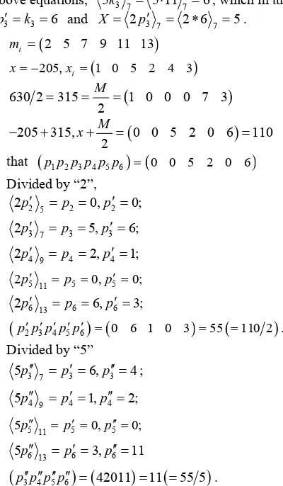
Example 4-3. For convenient comparison of the pro-posed TRD algorithm to other schemes such as appeared in [14], we take the same numerical example in [11]. Let the moduli set



m m m m m m₁, ₂, ₃, ₄, ₅, ₆

 

 2,5, 7,9,11,13



,

where



m m1, 2,m m3, 4



are regular moduli and



m m5, 6



2 5

M  

are redundant moduli. Then 7 9 630

k   

630 1

M M M 

, Mr 11 13 143 , 43 90090

 

kr k r , and



, 315,3

2 2

k k

p

M M

X  _ _ 

 

tions for correcting single residue digits errors are 1) Mr



m mi k s



maxi1, 2,3, or 4, s1, or 2,

4

k , The maximum

 

4 6 9 13 117 143

i k s r

m m_ m m     M

{2 } , 1, 2,3

M  m m m m i j

, and

2) r i j i j max , or 4,









3 4 3 4

The max 2 2

2 7 9 7 9

110 143 .

i j i j

r

m m m m m m m m

M

    

    

  

Thus the moduli set satisfies the necessary and suffi-cient conditions for correcting single errors digit. As-sume X  311



1, 4, 4, 4,8,1



and a single digit error

2 4

e  is introduced, then X



1,3, 4, 4,8,1



53743. After a polarity shift,



0,3, 4, 4, 4, 4 .



2 k p

M X X 

Follow the same procedures as shown in Example 4-2. CPRDD is applied for correction without the need for using a table.

1) Assign the moduli 4 as the reference moduli,

the following residue digit references and its correspon- 9

m 

ding CPRDD equations:

i i

ij _m ij

sk  d

m are obtained

14 2 1, 7 14 2 1;

d  k 

24 5 4, 4 24 5 4;

d  k 

34 7 0, 2 34 7 0;

d  k 

45 11 7, 2 45 11 7;

d  k 

46 13 3, 4 46 13 3.

d  k 

2) Choose two highest digit difference as one pair for equal target race distance e.g.

45 11 46 13

2k 7 and 4k 3. Then the true primary

RDD equations are

45 1 11

2k 11p 7 (4-11),

And 4k4613p2 13 3 (4-12),

where 1 and are selected so that the two RDD are

equal distances.

p p2

3) Eliminating k terms in Equation’s (4-11) and (4-12) by putting k45k46



1

 

2



22p  13p 11, ₁ 11 13



2



22

p

p   where

2 11

p  , then 1

11 143 7 22 p    .

4) Substituting p1 and p2 into equations (4-9) and (4-10)

respectively, we have 2k45     11 7 7 70, then

45 35

k   , and 4k46  13 11 3, also,

46

143 3 35 4

k     .

