Load Balancing Algorithm In Task Scheduling Process Using Cloud Computing

© 2016, IRJET | Impact Factor value: 4.45 | ISO 9001:2008 Certified Journal

| Page 3321

LOAD BALANCING ALGORITHM IN TASK SCHEDULING PROCESS USING

CLOUD COMPUTING

*1

_{Ms. Saranya G, *}

_{Mr. Srinivasan J}

_.

*1

_{M.Phil Research Scholar, Department of Computer Science Adhiparasakthi College of Arts and Science,}

Kalavai, TamilNadu, India

*

_{Assistant Professor, Department of Computer Science, Adhiparasakthi College of Arts and Science, Kalavai,}

TamilNadu, India

---***---Abstract

virtualization, distributed computing, networking, software and web services. A cloud consists of several elements such as clients, datacenter and distributed servers. It includes fault tolerance, high availability, scalability, flexibility, reduced overhead for users, reduced cost of ownership, on demand services etc. Central to these issues lies the establishment of an effective load balancing algorithm. The load can be CPU load, memory capacity, delay or network load. Load balancing is the process of distributing the load among various nodes of a distributed system to improve both resource utilization and job response time while also avoiding a situation where some of the nodes are heavily loaded while other nodes are idle or doing very little work. Load balancing ensures that all the processor in the system or every node in the network does approximately the equal amount of work at any instant of time. This technique can be sender initiated, receiver initiated or symmetric type (combination of sender initiated and receiver initiated types).Our objective is to develop an effective load balancing algorithm using to maximize or minimize different performance parameters (throughput, latency for example) for the clouds of different sizes (virtual topology depending on the application requirement).

Key Words:

Foraging Algorithm, Active Clustering Data communications and Transmission

I. INTRODUCTION

Cloud computing is an on demand service in which shared resources, information, software and other devices are provided according to the clients requirement at specific time. It’s a term which is generally used in case

of Internet. The whole Internet can be viewed as a cloud. Capital and operational costs can be cut using cloud computing. Cloud vendors are based on automatic load balancing services, which allowed entities to increase the number of CPUs or memories for their resources to scale with the increased demands.[2] This service is optional and depends on the entity's business needs. Therefore load balancers served two important needs, primarily to promote availability of cloud resources and secondarily to promote performance. According to the previous section Cloud computing will use the dynamic algorithm, which allows cloud entities to advertise their existence to presence servers and also provides a means of communication between interested parties. This solution has been implemented into the IETF’s RFC3920 - Extensible Messaging and Presence Protocol abbreviated as XMPP[3].

Fig : A cloud is used in network diagrams to depict the Internet

© 2016, IRJET | Impact Factor value: 4.45 | ISO 9001:2008 Certified Journal

| Page 3322

technique that facilitates networks and resources by providing a maximum throughput with minimum response time. Dividing the traffic between servers, data can be sent and received without major delay. Different kinds of algorithms are available that helps traffic loaded between available servers [2B]. A basic example of load balancing in our daily life can be related to websites. Without load balancing, users could experience delays, timeouts and possible long system responses. Load balancing solutions usually apply redundant servers which help a better distribution of the communication traffic so that the website availability is conclusively settled[5]. There are many different kinds of load balancing algorithms available, which can be categorized mainly into two groups. The following section will discuss these two main categories of load balancing algorithms.

1.1. LOAD BALANCERS

The « Load Balancer » systems allow you to create an infrastructure able to distribute the workload balancing it between two or more Cloud Servers. You can therefore shape your infrastructure to allow it to sustain activity peaks, optimize the allocation of resources and ensure a minimal response time. Using a load balancer is recommended in all cases whether you require one or more of the following:

• High traffic/request peaks • Guarantee of service continuity’s • Specialization of servers

To be able to balance the workload, you need at least two or more Cloud Servers in the same private network (VLAN). Aruba allows you to configure your load balancers, and its connections, directly from the Control Panel, with just a few clicks, easily and quickly[10][11]. It is very easy to configure your load balancers for the main protocols which are HTTP, HTTPS and TCP. You will then need to select the algorithm for the routing of the workload between Least Connection and Source.

Fig: Load Balancer

Cloud computing is a vast concept. Many of the algorithms for load balancing in cloud computing have been proposed. Some of those algorithms have been overviewed in this thesis. The whole Internet can be considered as a cloud of many connections less and connection oriented services [7]. So the divisible load scheduling theory for Wireless networks described in can also be applied for clouds. The performance of various algorithms have been studied and compared

.

II. RELATED WORK

A dynamic load balancing algorithm assumes no previous knowledge about job actions or the global state of the system, i.e., load balancing decisions is exclusively based on the existing or current status of the system [1]. In the distributed one, the dynamic load balancing algorithm is executed by all nodes present in the system and the task of load balancing is shared among them. The interaction among nodes to realize load balancing can take two forms:

1) Cooperative 2) Non-cooperative.

In the cooperative, the nodes work side by-side to attain a common goal, for example, to advance the overall response time,[2] etc. In the non-cooperative, every node works independently in the direction of a goal local to it, for example, to advance the response time of a local task [4]. Dynamic load balancing algorithms having distributed nature, frequently produce more messages than the non-distributed ones because, each of the nodes in the system is required to interact with every other node. The advantage, of this is that even if one or more nodes in the arrangement fail, it will not cause the total load balancing process to stop; it instead would influence the system performance to a little extent. In non-distributed type, either one node or a group of nodes perform the task of load balancing. Dynamic load balancing algorithms of non-distributed nature can get two forms:

1) Centralized 2) Semi-distributed.

© 2016, IRJET | Impact Factor value: 4.45 | ISO 9001:2008 Certified Journal

| Page 3323

compared to the semi-distributed case. However, centralized algorithms can create a bottleneck in the system at the central node and also the load balancing process is rendered hopeless once the central node crashes[9][10]. Therefore, this algorithm is mainly suited for networks with small size. Balancing technique.

2.1 EXISTING LOAD BALANCING ALGORITHMS

• Round Robin: In this algorithm, the processes are

divided between all processors. Each process is handed over to the processor in a round robin order. The process allotment order is maintained in the vicinity independent of the allotments from remote processors [6]. However the work load distributions between processors are the same but the job processing time for dissimilar processes are not same. So by any point of time some nodes may be greatly loaded and others wait at leisure. This algorithm is frequently used in web servers where http requests are of a like nature and scattered likewise.

•

• Connection Mechanism: Load balancing

algorithm can as well be based on least connection mechanism which is a component of dynamic scheduling algorithm[3]. It requires counting the number of connections for each server dynamically to approximate the load. The load balancer keeps track of the connection number of each server. The number of link adds to when a new connection is sent out to it, and decreases the number when connection terminates or timeout happens. A Task Scheduling Algorithm Based on

• Load Balancing: This is discussed a two-level

task scheduling method based on load balancing to convene dynamic requirements of users and obtain high resource utilization[8]. It accomplishes load balancing by first mapping tasks to virtual machines and then virtual machines to host resources by this means improving the task response time, resource consumption and overall performance of the cloud computing environment.

• Randomized: Randomized algorithm is of type

static in nature. In this algorithm a process can be handled by a particular node n with a probability p. The process allocation order is preserved for each processor independent of allotment from remote processor[5]. This algorithm facilitates well in case of processes that are equal loaded. On the other hand, trouble arises when loads are of different computational complexities.

Randomized algorithm does not keep up deterministic approach. It facilitates well while Round Robin algorithm generates overhead for process queue[8].

2.2 SERVICES PROVIDED BY CLOUD COMPUTING

1. Software as a Service (SaaS)

In SaaS, the user uses different software applications from different servers through the Internet. The user uses the software as it is without any change and do not need to make lots of changes or doesn’t require integration to other systems. The provider does all the upgrades and patching while keeping the infrastructure running[6].

Fig : Software as a service (SaaS)

2.Platform as a Service (PaaS)

PaaS provides all the resources that are required for building applications and services completely from the Internet, without downloading or installing software. PaaS services are software design, development, testing, deployment, and hosting. Other services can be team collaboration, database integration, web service integration, data security, storage and versioning etc[6].

© 2016, IRJET | Impact Factor value: 4.45 | ISO 9001:2008 Certified Journal

| Page 3324

It is also known as Infrastructure as a Service (IaaS). It offers the hardware as a service to an organization so that it can put anything into the hardware according to its will[5].

HaaS allows the user to "rent" resources as

• Server space

• Network equipment • Memory

• CPU cycles • Storage space

Fig : Hardware as a Service (HaaS)

III. SYSTEM IMPLEMETNATION

3.1 LOAD BALANCING

It is a process of reassigning the total load to the individual nodes of the collective system to make resource utilization effective and to improve the response time of the job, simultaneously removing a condition in which some of the nodes are over loaded while some others are under loaded. A load balancing algorithm which is dynamic in nature does not consider the previous state or behavior of the system, that is, it depends on the present behavior of the system. The important things to consider while developing such algorithm are : estimation of load, comparison of load, stability of different system, performance of system, interaction between the nodes, nature of work to be transferred, selecting of nodes and many other ones. This load considered can be in terms of CPU load, amount of memory used, delay or Network load.

Static load balancing: This is the basic method of load balancing. In this method the performance of the workers is determined at the commencement of execution. Then depending upon their performance the work load is distributed in the start. The workers compute their assigned work and submit their result to the master.

Dynamic load balancing: Dynamic load balancing determines the distribution of workload at run-time. The master assigns new task to the worker depending on the recent information collected. Since the workload distribution is done during runtime, it may give better performance. But the performance gained is at the cost of overhead associated with communication. So, the overhead associated should be in reasonable limit to achieve better performance

Network load balancing: Assume that you are running a website on Apache and you are starting to get a high enough level of traffic and load that you need to add additional Apache instances to help respond to this load. You can add additional Google Compute Engine instances and configure load balancing to spread the load between these instances. In this situation, you would serve the same content from each of the instances. As your site becomes more popular, you would continue increasing the number of instances that are available to respond to requests.

HTTP(S) load balancing: The network load balancing scenario above scales well for a single region, but to extend the service across regions, you would need to employ unwieldy and sometimes problematic solutions. By using HTTP(S) load balancing in this situation, you can use a global IP address that is a special IP that can intelligently route users based on proximity. You can increase performance and system reliability for a global user base by defining a simple topology.

Server Load Balancing: The Thunder Series and AX Series advanced server load balancing and flexible health monitoring capabilities provide application availability and reliability. The core of A10 ADC platform covers a wide range of options for load balancing methods and health checks. Comprehensive IPv4 and IPv6 support across all models maximizes options for current and future deployment.

© 2016, IRJET | Impact Factor value: 4.45 | ISO 9001:2008 Certified Journal

| Page 3325

In complex and large systems, there is a tremendous need for load balancing. For simplifying load balancing globally (e.g. in a cloud), one thing which can be done is, employing techniques would act at the components of the clouds in such a way that the load of the whole cloud is balanced. For this purpose, we are discussing three types of solutions which can be applied to a distributed system: honeybee foraging algorithm, a biased random sampling on a random walk procedure and Active Clustering.

Fig : deployment scenario with IP load balancers serving both directions for incoming and outgoing

requests in a cluster

4.1 HONEY BEE FORAGING ALGORITHM

This algorithm is derived from the behavior of honey bees for finding and reaping food. There is a class of bees called the forager bees which forage for food sources, upon finding one, they come back to the beehive to advertise this using a dance called waggle dance. The display of this dance, gives the idea of the quality or quantity of food and also its distance from the beehive. Scout bees then follow the foragers to the location of food and then began to reap it. They then return to the beehive and do a waggle dance, which gives an idea of how much food is left and hence results in more exploitation or abandonment of the food source.

The standard honey Bees Algorithm

1 for i=1,…,ns

i. scout[i]=Initialise_scout(

ii. lower_patch[i]=Initialise_flower_patch(scout[i])

2 do until stopping_condition=TRUE

i Recruitment()

iii. for i =1,…,nb

• flower_patch[i]=Local_search(flower_patc h[i])

• flower_patch[i]=Site_abandonment(flowe r_patch[i])

• flower_patch[i]=Neighbourhood_shrinkin g(flower_patch[i])

iv. for i = nb,…,ns

• flower_patch[i]=Global_search(flower_pat ch[i])}

As mentioned, the Bees Algorithm is an optimization algorithm inspired by the natural foraging behavior of honey bees to find the optimal solution pseudo code for the algorithm in its simplest form. The algorithm requires a number of parameters to be set, namely: number of scout bees (n), number of sites selected out of n visited sites (m), number of best sites out of m selected sites (e), number of bees recruited for best e sites (nep), number of bees recruited for the other (m-e) selected sites (nsp), initial size of patches (ngh) which includes site and its neighborhood and stopping criterion. The algorithm starts with the n scout bees being placed randomly in the search space. The fatnesses of the sites visited by the scout bees are evaluated in step 2.

v. Initialize population with random solutions.

vi. Evaluate fitness of the population.

vii. While (stopping criterion not met) //Forming new population.

viii. Select sites for neighborhood search.

ix. Recruit bees for selected sites (more bees for best e sites) and evaluate fit nesses.

x. Select the fittest bee from each patch.

xi. Assign remaining bees to search randomly and evaluate their fatnesses’.

xii. End While.

© 2016, IRJET | Impact Factor value: 4.45 | ISO 9001:2008 Certified Journal

| Page 3326

Techniques

4.2 Primary Scheduling Algorithm

There are M equal-sized independent tasks to be scheduled under the bandwidth-bounded cloud- computing environment. In order to minimize the total time (T) needed to finish all tasks, the scheduling node P0 needs to decide how many tasks should be specifically allocated and transferred to each VM. In order to achieve the optimized task allocation, we formulate a nonlinear programming model for the task-scheduling problem with the following constraints:

1. Ensures that the total number of tasks executed by all nodes is equal to M, where xi denotes the number of tasks allocated to node Pi.

2. Ensures that the number of tasks allocated to each of VMs is less than or equal to M.

3. Ensures that each VM node has computing power and bandwidth greater than 0.

4. Ensures that the execution of algorithm will not be misled and will not violate the real situation when task execution time wi is less than the task transmission time 1/bi. In such case, there will certainly exist the state that the previous task is already finished; however, the next task is yet to come. When that happens, VM could do nothing but wait. As such waiting unavoidably exists, the way to handle the waiting in the model is to append the time difference to execution time. In other words, as the execution waits until transmission ends, the scheduling strategy regards execution time wi the same as transmission time 1/bi. The preceding equation is the case when wi is less than 1/ bi; The algorithm is deployed on Broker and works out the optimized task allocation scheme on the basis of information of VM (computing power and bandwidth) and submits the optimized scheme to the Datacenter, so that the Datacenter allocates tasks to VMs according to the optimized task allocation scheme.

4.3 Modified Scheduling Algorithm

In BATS, if a set of tasks that represent a divisible load application is submitted to the Datacenter, then obtain computing power and bandwidth of VMs owned by Broker, obtain information about tasks, build a nonlinear programming model, and solve the model and obtain the optimized task allocation scheme A that determines proper number of tasks assigned to each VM. In each iteration, one VM is bound the proper number of tasks. Then, the Broker sets bandwidth used in task transmission and transfers task on the basis of the bandwidth. T.

i. Procedure BATS ()//scheduling algorithm of Broker

ii. If (Task_Submitted())//if there is a set of tasks submitted

iii. GetVmInfo()//get computing power and bandwidth of VMs owned by Broker

iv. GetTaskInfo()//get information about tasks, including total number and size

v. Build_Model(model)//build a nonlinear programming model A=Solve(model)//solve the model and obtain the optimized task allocation scheme

vi. A End If

vii. While (Exist_Idle())//when there is a idle VM in virtual machine list vmlist

viii. vmi=GetNextIdle(vmlist)//get next idle virtual machine vmi from vmlist

ix. Ti=GetTaskNum(A)//get the number of tasks, Ti, allocated to vmi in A

x. Bind(A, vmi)//bind Ti tasks to vmi SetBandwidth(vmi, b′i)// set bandwidth used in task transmission: b′i=xi/(T-wi)

xi. End while

xii. Submit ()//concurrently send tasks with new bandwidth

© 2016, IRJET | Impact Factor value: 4.45 | ISO 9001:2008 Certified Journal

| Page 3327

RESULT AND EVAILATION RESULT

Here we consider the following two cases. In the first case the measurement and reporting time is plotted against the number of slaves corresponding to a master, where the link speed b is varied and measurement speed a is fixed. In the second case, the measurement and reporting time is plotted against the number of slaves corresponding to master, where link speed b is fixed and measurement speed a is varied. Load balancer is a key element in resource provisioning for high available cloud solutions, and yet its performance depends on the traffic offered load. We develop a discrete event simulation to evaluate the performance with respect to the different load points. The performance metrics were the average waiting time inside the balance as well as the number of tasks. The performance study includes evaluating the chance of immediate serving or rejecting incoming tasks.

The users execute their processes on their hosts, and the random arrival of newly created processes can make some systems overloaded and some systems under loaded or idle. To overcome this problem at runtime, load balancing is used. Load Balancing is used in distributed memory multiprocessor to balance the workload among workstations automatically at execution time. Ideally we always wish all processors to be executing continuously on the tasks to give a superior performance.

The case when the inverse measuring speed a is varied from 1 to 2 at an interval of 0.3 and the inverse link speed b is fixed to be 0.2. The result confirms that the measurement time approaches b1Tcm, which in this case is 0.2, as N approaches infinity.

Fig : Measurement/report time versus number of slaves corresponding to master and variable inverse link speed b for single level tree network with master

and sequential reporting time.

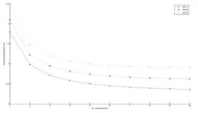
The measurement/report time is plotted against the number of slaves corresponding to a master for the simultaneous measurement start simultaneous reporting termination case. The value the inverse link speed b is varied from 0 to 1 at an interval of 0.3 while the inverse measuring speed a is fixed to be 1.5. In this case the minimum finish time decreases as the number of slaves

under a master in the network is increased. This assumes that the communication speed is fast enough to distribute the load to all the slaves under a master.

Fig : Measurement/report time versus number of slaves under a master and variable inverse link speed

b for single level tree network with master

Fig : Measurement/report time versus number of slaves under a master and variable inverse measuring

speed a for single level tree network with master

The comparison between the

© 2016, IRJET | Impact Factor value: 4.45 | ISO 9001:2008 Certified Journal

| Page 3328

finishing time can be decreased significantly in case of simultaneous measurement start and simultaneous reporting termination by increasing the no. of slaves under a single master computer.

CONCLUSION

In this paper, we presented in till now we have discussed on basic concepts of Cloud Computing and Load balancing and studied some existing load balancing algorithms, which can be applied to clouds. In addition to that, the closed-form solutions for minimum measurement and reporting time for single level tree networks with different load balancing strategies were also studied. The performance of these strategies with respect to the timing and the effect of link and measurement speed were studied. A comparison is also made between different strategies.

FUTURE WORK

Cloud Computing is a vast concept and load balancing plays a very important role in case of Clouds. There is a huge scope of improvement in this area. We have discussed only two divisible load scheduling algorithms that can be applied to clouds, but there are still other approaches that can be applied to balance the load in clouds. The performance of the given algorithms can also be increased by varying different parameters.

REFERENCES:

[1]. Bhasker Prasad Rimal, Eummi Choi, Lan Lump (2009) “A Taxonomy and Survey of Cloud Computing System”, 5th International Joint Conference on INC, IMS and IDC, IEEE Explore 2527Aug 2009, pp. 44-51

[2]. Bhathiya, Wickremasinghe.(2010)”Cloud Analyst: A Cloud Sim-based Visual Modeller for Analysing Cloud Computing Environments and Applications”

[3] C.H.Hsu and J.W.Liu(2010) "Dynamic Load Balancing Algorithms inHomogeneous Distributed System," Proceedings of The 6thInternational Conference on Distributed Computing Systems, , pp. 216-223.

[4] Calheiros Rodrigo N., Rajiv Ranjan, César A. F. De Rose, Rajkumar Buyya (2009): “CloudSim: A Novel Framework for Modeling and Simulation of Cloud Computing” Infrastructures and Services CoRR abs/0903.2525: (2009)

[5] Carnegie Mellon, Grace Lewis(2010) “Basics About Cloud Computing” Software Engineering Institute September 2011

[6] Cary Landis, Dan Blacharski, “Cloud Computing Made Easy”, Version 0.3

[7] “CloudSim: A Framework for Modeling and Simulation of Cloud Computing Infrastructures and Services, The Cloud Computing and Distributed Systems” (CLOUDS) Laboratory, University of Melbourne, (2011) available from: http://www.cloudbus.org/cloudsim/

[8] G. Khanna, K. Beaty, G. Kar, and A. Kochut,(2006)

“Application Performance Management in Virtualized Server Environm,” in Network Operationsand Management Symposium, (2006). NOMS (2006). 10th IEEE/IFIP, pp 373– 381.

[9] Jaspreet kaur (2012),”Comparison of load balancing algorithms in a Cloud” International Journal of Engineering Research and Applications(IJERA) ISSN: 2248-9622 www.ijera.comVol. 2, Issue 3,pp.1169-1173