RULES REDUCTION AND OPTIMIZATION OF FUZZY LOGIC MEMBERSHIP FUNCTIONS FOR INDUCTION MOTOR SPEED CONTROLLER

5012

OPTIMAL COMPLEX WEIGHTS ANTENNA ARRAY WITH

EFFICIENT FUZZY PARTICLE SWARM OPTIMIZATION

ALGORITHM

BRAHIMI MOHAMED,KADRIBOUFELDJA

1_{Smart Grids & Renewable Energies Laboratory, University Tahri Mohamed of Bechar, 08000, Algeria}

E-mail: [email protected], [email protected]

ABSTRACT

In this article, a stochastic optimization technique called fuzzy particle swarm optimization (FPSO) is presented to determine an optimum set of microstrip antenna arrays excitation weights (amplitude and phase), the use of the fuzzy controller allows to dynamically adjust its parameters such as, the inertia weight and acceleration coefficients in order to produce an optimal pattern of the antenna array able to approach a desired pattern. Simulation results are proposed to compare with published results to verify the effectiveness of the suggest method for both linear and planar array.

Keywords: Fuzzy Controller, Linear Array, Particle Swarm Optimization, Pattern Synthesis, Planar

Array.

1. INTRODUCTION

The domain of wireless communication has witnessed an explosive growth in the last years, indeed the creation of new technologies which ensure the offered services and products to ever more the customer’s requirements [1]. For communications using electromagnetic waves propagation in the free space, the antenna is an essential element to ensure the information emission and reception. The microstrip antennas are designed to meet the requirements of this technological evolution, which also tends towards the miniaturization of electronic devices and telecommunications systems. Their small size, performance and flexibility make them particularly adaptable to mobile machinery (satellite, aircraft, boat) and their flexibility, enabling them to conform to any form of surface (flat or conformal), these antennas have proved their effectiveness and tend to replace conventional antennas definitely [2]. Their array association, which is thoroughly researched, also allows their performance to be improved, and to perform particular functions that are better suited to certain types of applications, such as: depointage, electronic scanning and rejection of jammers [3].

In this field, many analytical and numerical methods have been developed to try to synthesize a desired radiation pattern. Among these methods, we propose to solve the synthesis problem using methods based on the concept of particles swarm

[4]. This algorithm (PSO) is an evolutionary algorithm based on the swarm intelligence [5], which can be used to solve complex global optimization problems. Currently, the algorithm and its variations are applied to many practical problems [6]. It has many outstanding advantages, such as fast convergence, simple computation and easy implementation.

Although, the basic version of PSO algorithm suffers from problems such as prematurity, limited searching scope and trend to converge to local extremes and similar to other evolution algorithms.

To surmount these problems, many researchers have employed methods to adapt PSO parameters, in order to adjust the parameters of the PSO algorithm, a fuzzy controller was designed. We present in this paper the synthesis of the complex radiation pattern of a linear and planar antenna array with probe feed by optimizing the amplitude and phase excitations. The desired radiation pattern is specified by a narrow beam pattern with a beam width of 8 degrees and maximum side lobe level of -20 dB pointed at 15°.

5013 parameters so that the array meets the user requirements according to precise specifications?

2. THE PSO ALGORITHM

Particle swarm optimization (PSO) is a population based stochastic optimization technique developed by Kennedy and Eberhart [4,7]. It exhibits some evolutionary computation attributes:

 It is initialized with a population of random solutions.

 It searches for optima by updating generations.

 Updating is based on previous generations.

In PSO, the potential solutions, called particles, fly through the problem space by following the current optimum particles. The updates of the particles are accomplished according to the following equations. Equation (1) calculates a new velocity for each particle (potential solution) based on its previous velocity (Vid), the particle's

location at which the best fitness has been achieved (Pid, or Pbest) so far, and the best particle among the

neighbors(Pnd, or Gbest) at which the best fitness has

been achieved so far. Equation (2) updates each particle's position in the solution hyperspace. Where ω is the inertia weight, R1 and R2 are

independently generated in the range [0, 1], and C1,

C2 are acceleration coefficients.

) .( . ) .( .

. id 1 1 id id 2 2 nd id

id V C R P X C R P X

V      (1)

id id

id X V

X   (2)

A basic PSO algorithm can be described as follows [8]:

Step1: Specify the parameters for the PSO.

Step2: Initialize population of particles having

positions and velocities.

Step3: Calculate the fitness of each particle.

Step4: Until a stopping criterion is met, update the

particle velocity according to equation (1), and the particle position according to equation (2).

Step5: At the end of the iterative process, the best

solution is achieved.

3. FUZZY PARTICLE SWARM

OPTIMIZATION ALGORITHM

The particle swarm optimization parameters namely, the inertia weight (ω) as well as the acceleration coefficients (C1 and C2) can be

adaptively adjusted according to the control information translated from fuzzy logic controller (FLC) during the search process, through an algorithm called a fuzzy particle swarm

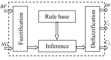
optimization(FPSO). This algorithm is intended to improve the performance of PSO; a fuzzy system will be employed to adjust the PSO parameters [9]. During the evolution of algorithm, it is noticeable that, when the best fitness is low at the end of the run in the optimization of a minimum function, low inertia weight and high acceleration coefficients are often preferred [11]. When the best fitness is stuck at one value for a long time, number of generations for unchanged best fitness is large. The system is often stuck at a local minimum, so the system should probably concentrate on exploiting rather than exploring. That is, the inertia weight should be increased and acceleration coefficients should be decreased. Based on this kind of knowledge, a fuzzy system is developed to adjust the inertia weight, and acceleration coefficients with best fitness (BF) and number of generations for unchanged best fitness (NG) as the input variables, and the inertia weight (ω) and acceleration coefficients (C1 and C2) as output variables (Figure

1).

Figure 1: Structure of fuzzy controller

Where the range of BF and NG are [0, 1]. The value for ω is bounded between 0.2 and 1.2 and the values of C1 and C2 are bounded between 1.0

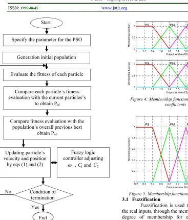
and 2.0 (Figure (3-5)).The fuzzy particle swarm optimization algorithm (FPSO) progress is shown by the flowchart shown in (Figure 2).

The membership functions of inputs and outputs of FPSO model are shown in figures (3-5). The fuzzy system consists of four principal components (Figure 1) [11]: fuzzification, fuzzy rules, fuzzy reasoning and defuzzification, which are described as below:

Rule base

Inference

Defuzzification

Fuzzificatio

n



1 C

2 C NG

5014 Figure 2: Flowchart of fuzzy PSO algorithm

Each rule represents a mapping from the input space to the output space.

0 0.1 0.2 0.3 0.4 0.5 0.6 0.7 0.8 0.9 1

0 0.5 1

Input variable (Best fitness)

M

em

be

rs

hi

p

func

tion PS PM PB PR

0 0.1 0.2 0.3 0.4 0.5 0.6 0.7 0.8 0.9 1

0 0.5 1

Input variable ((Number of generation for unchanged best fitness)

Me

mb

er

sh

ip

f

un

ct

io

n _{PS PM PB PR}

Figure 3: Membership functions of best fitness and number of generation for unchanged best fitness

1 1.1 1.2 1.3 1.4 1.5 1.6 1.7 1.8 1.9 2

0 0.5 1

Output variable (C1))

M

em

be

rs

hi

p

func

tion PS PM PB PR

1 1.1 1.2 1.3 1.4 1.5 1.6 1.7 1.8 1.9 2

0 0.5 1

Output variable (C2))

Me

mb

er

sh

ip

f

un

ct

io

n _{PS PM PB PR}

Figure 4: Membership functions for acceleration coefficients

0.2 0.3 0.4 0.5 0.6 0.7 0.8 0.9 1 1.1 1.2

0 0.2 0.4 0.6 0.8 1

Output variable (W))

M

em

be

rs

hi

p

func

tion

PS PM PB PR

Figure 5: Membership functions for inertia weight

3.1 Fuzzification

Fuzzification is used to associate each of the real inputs, through the membership functions, a degree of membership for each fuzzy subsets defined on the entire speech. The purpose of the fuzzification is to transform the input variables to variables "Linguistic" or fuzzy variables. Thus, in this example, they will be qualified to Little (P), Medium (M) and Large (L).

3.2 Fuzzy rules

The Mamdani-type fuzzy rule is used to formulate the conditional statements that comprise fuzzy logic. The fuzzy rules in Tables 1, 2 and 3 are used

to adjust the inertia weight (ω) and acceleration coefficients (C1 and C2), respectively.

Table 1: Fuzzy rules for inertia weight (ω). ω

BF NUMBER_GEN

PS PM PB PR

PS PS PM PB PB

PM PM PM PB PR

PB PB PB PB PR

PR PB PB PR PR

Updating particle’s velocity and position

by eqs (1) and (2)

Fuzzy logic controller adjusting



Condition of termination No

Yes

Specify the parameter for the PSO

Generation initial population

Evaluate the fitness of each particle

Compare each particle’s fitness evaluation with the current particles’s

to obtain Pid

Compare fitness evaluation with the population’s overall previous best

obtain Pnd

Start

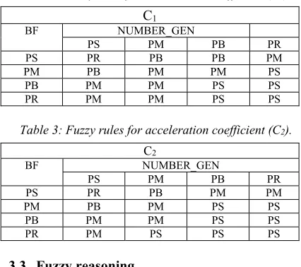
5015 Table 2: Fuzzy rules for acceleration coefficient (C1).

C1

BF NUMBER_GEN

PS PM PB PR

PS PR PB PB PM

PM PB PM PM PS

PB PM PM PS PS

PR PM PM PS PS

Table 3: Fuzzy rules for acceleration coefficient (C2). C2

BF NUMBER_GEN

PS PM PB PR

PS PR PB PM PM

PM PB PM PS PS

PB PM PM PS PS

PR PM PS PS PS

3.3 Fuzzy reasoning

The fuzzy control strategy is used to map from the given inputs to the outputs [10]. Mamdani’s fuzzy inference method is used in this study [12]. The AND operator is typically used to combine the membership values for each fired rule to generate the membership values for the fuzzy sets of output variables in the consequent part of the rule. Since there may be several rules fired in the rule sets, for some fuzzy sets of the output variables there may be different membership values obtained from different fired rules.

These output fuzzy sets are then aggregated into a single output fuzzy set by OR operator. That is to take the maximum value as the membership value of that fuzzy set.

3.4 Defuzzification

To obtain a deterministic control action, a defuzzification strategy is required. The method of centroid (center-of-sums) is used as shown below:

 

 





 



i Bi y

n

i Bi

dy

y

dy

y

y

y

1 1

.





(3)

Defuzzified value is directly acceptable values of ω, C1 and C2 parameters, where the input

for the defuzzification process is a fuzzy set: μBi(y)

(the aggregate output fuzzy set) and the output is a single number y.

4. SIMULATION RESULTS

Many applications require radiation characteristics that may not be achievable by a

single element. It may, however, be possible that an aggregate of radiating elements in an electrical and geometrical arrangement (an array) will result in the desired radiation characteristics. The arrangement of the array may be such that the radiation from the elements adds up to give a radiation maximum in a particular direction or directions, minimum in others, or otherwise as desired. Two typical examples of arrays are presented in this paper [1]:

4.1 Linear array

The array pattern can approach the desired template by adjusting the exciting current amplitude and phase shift of each element in a uniform linear array with N isotropic elements. From the antenna theories, the far field pattern of a uniform linear array is:















 N

i i i i

X k j a F f F

1 0

max

cos sin exp

) , ( ) ,

(       (4)

Where

f(θ,φ) is the radiation pattern, N is the number of elements,

k0: wave number k0 = 2π/λ, θ: angular direction,

ai, ψi: amplitude and phase of the complex

excitation power.

The numerical results reported in this section were obtained by the implementation of the both algorithms, FPSO and PSO for the synthesis of uniformly spaced linear array constituted with 16 rectangular microstrip antennas (Figure 6).

Figure 6: Linear antenna array

In the example of simulation introduced, the excitation weights (amplitudes and phases) are optimized to produce a desired radiation pattern specified by a symmetrical narrow beam pattern with a beam width of 8 degrees and maximum side lobe level of -20dB. The simulation parameters are selected for PSO: the inertia weight equal to 0.7 and acceleration coefficients C1 and C2 equal to

1.48, which is analogous to Clerc’s setting [5].

1



M

-1



2 3

d

N

Y

5016 However in FPSO, these parameters are adjusting by the fuzzy logic controller (FLC), with a population size equal to 30 individuals. Figure 7 shows the radiation patterns of linear antenna array synthesis by the optimization of amplitude and phase excitation coefficients using the both of FPSO and PSO for scanning angle of 15 degrees. From this figure, it is clearly seen that the radiation pattern acquired by FPSO meets better the desired pattern than the obtained by the PSO. The maximum side lobe level obtained of the FPSO pattern is -31.85 dB, whereas that of PSO is-22.19 dB (Figure 7).

-100 -80 -60 -40 -20 0 20 40 60 80 100

-100 -90 -80 -70 -60 -50 -40 -30 -20 -10 0

theta [degree]

A

m

pl

itude

FPSO PSO fd

Figure 7: Radiation patterns of a linear array with 16 elements pointed at 15 degrees optimized by both FPSO

and PSO

0 100 200 300 400 500 600

0 0.1 0.2 0.3 0.4 0.5 0.6 0.7 0.8

Iterations

Fi

tn

es

s

FPSO PSO

Figure 8: Fitness evolution of FPSO and PSO algorithms

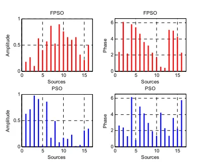
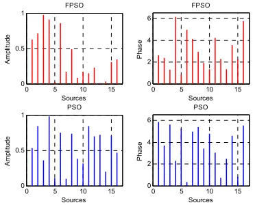
The optimized amplitude and phase excitation coefficients found by both optimized algorithm are illustrated in figure 9. The program was written and run in MATLAB (R2010a) on 2.3 GHz intel(R) core(TM) i3-2348M CPU with 4GB RAM

0 5 10 15

0 0.5 1

Sources

A

m

pl

itud

e

FPSO

0 5 10 15

0 2 4 6

Sources

Ph

as

e

FPSO

0 5 10 15

0 0.5 1

Sources

A

m

plit

ud

e

PSO

0 5 10 15

0 2 4 6

Sources

P

has

e

PSO

Figure 9: Optimized sources amplitude and phase excitations

We have chosen a suitable fitness functions that can guide the FPSO and PSO optimization toward a solution that meets the desired radiation pattern. The fitness function to be minimized is selected from the work of Chuan Lin [13] which is described by the equation below:

 

_{ }

 

0







 



F F S

A

A

Max

f



Where S is the space spanned by the angle θ excluding the main lobe and ρ represents the unknown parameter vector, such as element positions and phases. This objective function minimizes all the side lobe levels and maximizes the power in the main lobe located at θ=θ0.

From figure 8, the approached speed of the global optimal of FPSO is much quickly than that of PSO, and the fitness values of the best individuals of FPSO are almost lower than that of PSO in every population.

0 100 200 300 400 500 600

0.65 0.7 0.75 0.8

Iterations

In

er

tia

W

ei

gh

t W

FPSO PSO

5017

0 100 200 300 400 500 600

1.44 1.46 1.48 1.5 1.52 1.54 1.56 1.58 1.6

Iterations

A

cc

el

er

at

ion

C

oef

fic

ient

C

1

FPSO PSO

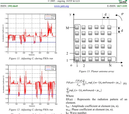
Figure 11: Adjusting C1 during PSOs run

0 100 200 300 400 500 600

1.46 1.47 1.48 1.49 1.5 1.51 1.52 1.53 1.54 1.55

Iterations

A

cc

el

er

ati

on

C

oe

ffi

ci

en

t C

2

FPSO PSO

Figure 12: Adjusting C2 during PSOs run The adjustment of the inertia weight and acceleration coefficients during the evolution process of the two algorithms (FPSO and PSO) are illustrated in figures (10-12).

4.2 Planar array

For a linear array, the synthesis is reduced to check the feed law on an axis, of number of elements fixed in advance, while in a planar array, the research synthesis’s are consisted of the complex weighting of the sources power supply in a plan [15]. This generalization of the planar array (Figure 13) is considered by replacing the direction θ by the pair of directions (θ, φ). Let us consider a planar antenna array constituted of MxN equally spaced rectangular antenna arranged in a regular rectangular array in the x-y plane, with an inter-element spacing of d=dx=dy=λ/2 (Figure 13), and whose outputs are added together to provided a single output.

Mathematically, the normalized array far-field pattern is given by:

Figure 13: Planar antenna array

 

_

_

_

_

 





0 1

max

0 1

,

( , ) exp 1 sin cos

. exp 1 sin cos

M

mn mn

i N

mn i

f

F I j m k dx j

F

j n k dy j

 

    

  





  

 





(6)

Where

f(θ,φ) : Represents the radiation pattern of an element.

Imn : Amplitude coefficient at element (m, n).

ψmn: Phase coefficient at element (m, n).

k0: Wave number.

The FPSO algorithm is able to model and to optimize the antennas arrays, by acting on radioelectric parameters of the feed law (amplitude and/or phase) of the radiating sources.

In that the synthesis of uniformly spaced planar array of 4x4 rectangular patch antennas is presented.

In our simulation, we have used the same parameters used in the linear array. The FPSO and PSO techniques are applied to sixteen (4×4) planar antenna array elements to produce radiation patterns shown in figure 14. Their type is rectangular microstrip antennas with 0.906 cm width and 1.186 cm long working at the frequency of 10 GHz.

From this figure (figure 14), it is noticed that the radiation pattern are contained within the limits imposed by the template and the maximum of side lobes level is lower than -20 dB in such way that the FPSO is better than PSO and reaches them respectively - 33.69 dB and -21.3 dB.

o

1

2

N

x

y

d



d

2

5018

-100 -80 -60 -40 -20 0 20 40 60 80 100

-100 -90 -80 -70 -60 -50 -40 -30 -20 -10 0

theta [degree]

A

m

pl

itude

FPSO PSO fd

Figure 14: Radiation patterns of a planar array with 16 elements pointed at 15 degrees optimized by both FPSO

and PSO

0 100 200 300 400 500 600

0 0.1 0.2 0.3 0.4 0.5 0.6 0.7 0.8 0.9 1

Iterations

Fi

tn

es

s

FPSO PSO

Figure 15: Fitness evolution of FPSO and PSO algorithms

The optimized amplitude and phase excitation coefficients obtained by both optimizing algorithms; are represented in figure 16.

Results of the adjusting of the inertia weight and acceleration coefficients during the evolution process are plotted in figures (17-19).

0 5 10 15

0 0.5 1

Sources

A

m

pl

itud

e

FPSO

0 5 10 15

0 2 4 6

Sources

Ph

as

e

FPSO

0 5 10 15

0 0.5 1

Sources

A

m

plit

ud

e

PSO

0 5 10 15

0 2 4 6

Sources

P

has

e

PSO

Figure 16: Optimized sources amplitude and phase excitations

0 100 200 300 400 500 600

0.65 0.7 0.75 0.8

Iterations

In

er

tia

W

ei

ght

W

FPSO PSO

Figure 17: Adjusting ω during PSOs run

0 100 200 300 400 500 600

1.45 1.46 1.47 1.48 1.49 1.5 1.51 1.52 1.53

Iterations

A

cc

el

er

at

ion

C

oef

fic

ient

C

1

FPSO PSO

Figure 18: Adjusting C1 during PSOs run

0 100 200 300 400 500 600

1.44 1.45 1.46 1.47 1.48 1.49 1.5 1.51 1.52

Iterations

A

cce

le

ra

tio

n

C

oe

ffi

ci

en

t C

2

FPSO PSO

Figure 19: Adjusting C2 during PSOs run

5. COMPARATIVE STUDY

To validate the capability and flexibility of the proposed method for synthesis of patterns arrays, two illustrative examples of simulation of microstrip antenna array have been considered. In the first example, the proposed technique FPSO is compared to GA [15] and PSO [16].

5019 inertia weight ω=0.3. For the genetic algorithm GA, the crossover probability Pc=1 and the mutation

probability Pm= 0.01.

Figure 20 shows the synthesis results of 16 linear antenna array with half wave length spacing obtained by the application of FPSO, GA and PSO, from this figure, the maximum side lobe level obtained by FPSO (-37.99 dB) is lower than GA(-20 dB) and PSO (-25.88 dB).

In the second example, 36 elements (6×6) are synthesized by FPSO compared also with GA [17] and PSO [18]. From results given by figure 21, it is clear that the proposed technique pattern achieve a maximum side lobe level of (-36.43 dB), as for the both technique GA and PSO set a maximum side lobe level of 20.56 dB) and (-22.82 dB) respectively.

-100 -80 -60 -40 -20 0 20 40 60 80 100

-100 -90 -80 -70 -60 -50 -40 -30 -20 -10 0

theta [degree]

A

m

pl

itude

FPSO PSO GA

Figure 20: Radiation patterns of a linear array with 16 elements pointed at 20 degrees optimized by FPSO, PSO

and GA

-100 -80 -60 -40 -20 0 20 40 60 80 100

-100 -90 -80 -70 -60 -50 -40 -30 -20 -10 0

theta [degree]

A

m

pl

itude

FPSO PSO GA

Figure 21: Radiation patterns of a planar array with 16 elements pointed at 30 degrees optimized by FPSO,PSO

and GA

Simulation results of this comparative study are given to show the effectiveness and the consistency of the FPSO algorithm by the tuning of its parameters in order to search for the optimum amplitude and phase excitation weights to minimize maximum side lobe level and steer the pattern main lobe in a desired direction (15, 20 and 40 degrees). Moreover, it can be noticed that FPSO is more robust than GA, since it has presented to avoid entrapment in local optima and improve the convergence speed and the accuracy in the array synthesis.

In this comparative study between the proposed algorithm and both algorithms PSO and GA published in the litterature, we took the same parameters for the three algorithms except that with the proposed algorithm, the parameters are not fixed and are readjusted by the fuzzy controller during optimization process. This adjustement of the parameters provides a good solution accuracy with a reasonable number of the fitness evaluation and efficient result compared to the results found by the two published algorithms.

6. CONCLUSION

The synthesis of antenna array with a specific radiation pattern, limited by several constraints, is highly a non linear optimization problem. Many evolutionary methods have been proposed for its solutions, one of these techniques includes the well-know particle swarm optimization (PSO) method. It is easy to implement, but it suffers from premature convergence and trapping in local minimum. For these reasons, a fuzzy logic controller has been implemented to adjust the control parameters on-line to dynamically adapt the PSO parameters to new situations. So the FPSO has been built for inducing exploitation/exploration relationships that avoid premature convergence problem and improve the final results by optimizing the parameters controlling the PSO like inertia weight and acceleration coefficients depending on the algorithm population. The simulation results demonstrate the good agreement between the synthesized pattern and the desired one obtained in case of FPSO than those while using PSO.

5020 REFRENCES:

[1] C. Balanis, “Antenna theory: analysis and design”, 1997, New Jersey: Wiley.

[2] W.H Kummer, “Basic Array Theory”,

Proceedings of IEEE, Vol. 80, No. 1, 1992, pp. 127-140.

[3] L.Merad, S.M. Meriah, and F.T. Bendimerad, “Modélisation et Optimisation par Les Réseaux de Neurones de Réseaux d’Antennes Imprimées”, Journées des Mathématiques Appliquées (JMA2000), Blida, November 13-14, 2000, pp. 53.

[4] J.Kennedy, and R.Eberhart, “Particle Swarm Optimization”, Proceedings of IEEE conference on neural networks, Vol. 4, 1995, pp.1942– 1948.

[5] M.Clerc, and J.Kennedy, “The Particle Swarm, Explosion, Stability, and Convergence in A Multidimensional Complex Space”, IEEE Transactions on Evolutionary Computation, Vol. 6, No. 4, 2002, pp.58-73.

[6] J.Robinson, and Y.R. Samii, “Particle Swarm Optimization in Electromagnetics”, IEEE Transactions on Antennas and Propagation, Vol. 52, No. 2, 2004, pp.397-407.

[7] R.C. Eberhart, and J. Kennedy, “A New Optimizer Using Particle Swam Theory”, Nagoya, Japan, 1995, pp. 3943.

[8] F. Marini, and B. Walczak, “Particle Swarm Optimization”, A Tutorial, Chemometrics and Intelligent Laboratory Systems, Volume 149, Part B, December 15, 2015, pp. 153–165 [9] T.D. Ping, and L.N. Qian, “Fuzzy Particle

Swarm Optimization Algorithm”, Artificial Intelligence, International Joint Conference, 2009, pp. 263-267.

[10] A.Abujasser, and H. Shaheen, “Multi-Objective Solution Based on Various Particle Swarm Optimization Techniques in Power Systems”,

Research Journal of Applied Sciences Engineering and Technology, Vol. 3, 2011, pp.519-532.

[11] J.R. Timonthy, “Fuzzy Logic with Engineering Applications”, 1997, Mc Graw-Hill, New York. [12] E.H. Mamdani, “Application of Fuzzy

Algorithms for The Control of A Dynamic Plant”, Proceedings of IEEE, Vol. 121, No. 12, 1974, pp.1585-1588.

[13] L. Chuan, A. Qing and Q.Feng1, “Synthesis of Unequally Spaced Antenna Arrays by A New Differential Evolutionary Algorithm”,

International Journal of Communication Networks and Information Security (IJCNIS), Vol. 1, No. 1, April 2009, pp. 20-25.

[14] B. Kadri, M. Boussahla, and F.T. Bendimerad, “Phase-Only Planar Antenna Array Synthesis with Fuzzy Genetic Algorithms”, International Journal of Computer Science Issues (IJCSI), Vol. 7, Issue 1, No. 2, January 2010, pp. 72-77. [15] A. Raniszewski, “Radiation Pattern Synthesis

for Radar Application Using Genetic Algorithm”, 21st _{International Conference on}

Microwave Radar and Wireless Communications (MIKON), May 9-11, 2016, pp. 1-4.

[16] Y.Y. Bai, S. Xiao, C. Liu, and B.Z. Wang, “A Hybrid IWO/PSO Algorithm for Pattern Synthesis of Conformal Phased Arrays”, IEEE Transactions on Antennas and Propagation, Vol. 61, No. 4, April 4, 2013, pp 2328-2332. [17] C.M. Seong, M.S. Kang, C.S. Lee, and D.C.

Park, “Conformal Array Pattern Synthesis on a Curved Surface with Quadratic Function using Adaptive Genetic Algorithm”, Proceedings of Asia-Pacific Microwave Conference (APMC), November 5-8, 2013, pp 167-169.