http://www.sciencepublishinggroup.com/j/ijsda doi: 10.11648/j.ijsd.20170304.15
ISSN: 2472-3487 (Print); ISSN: 2472-3509 (Online)
Challenges and Implications of Missing Data on the Validity
of Inferences and Options for Choosing the Right Strategy
in Handling Them
Nicholas Pindar Dibal
1, *, Ray Okafor
2, Hamadu Dallah
31
Department of Mathematical Sciences, University of Maiduguri, Maiduguri, Nigeria 2
Department of Mathematics, University of Lagos, Lagos, Nigeria 3
Department of Actuarial Science, University of Lagos, Lagos, Nigeria
Email address:
[email protected] (N. P. Dibal), [email protected] (R. Okafor), [email protected] (H. Dallah)
To cite this article:
Nicholas Pindar Dibal, Ray Okafor, Hamadu Dallah. Challenges and Implications of Missing Data on the Validity of Inferences and Options for Choosing the Right Strategy in Handling Them. International Journal of Statistical Distributions and Applications.
Vol. 3, No. 4, 2017, pp. 87-94. doi: 10.11648/j.ijsd.20170304.15
Received: September 19, 2017; Accepted: October 17, 2017; Published: November 20, 2017
Abstract:
Missing data in surveys and experimental research is a common occurrence which has serious implications on the validity of inferences. Advances in statistical procedures provides better and efficient methods of handling missing data yet many researches still handle incomplete data in ways that affects the results negatively. We review in detail the mechanisms that generates missingness, and the appropriate methods to account for the missing values to enable the researcher have adequate knowledge to make informed decision on the choice of method to account for missingness.Keywords:
Missing Data, Inference, Missingness Mechanisms, Ignorable, Non-Ignorable Missingness, Multiple Imputation1. Introduction
Missing values creates serious problems for researchers on the field and other data users during statistical analyses and data interpretation, especially when the assumption of ignorability of the missing data does not hold because most of statistical methods are not designed to handle incomplete data ([33]; [28]; [18]). Improper methods used to account for missing data usually results in biased estimate ([29]; [36]; [42]). Missing data are unobserved values, they occur when the actual data we intend to measure could not be measured for some reasons leaving us with incomplete data. Missing data is a common occurrence in surveys and experiments when something goes wrong for unanticipated reasons. Data may be missing for a wide range of reasons some of which can be partially controlled by the researcher while others are not. The ethical imperative that participation in any study is voluntary means that participants are free to skip any question on issues sensitive to them or even withdraw from the study whenever they wish thereby increasing the possibilities of missing values [1].
Missing values are unavoidable in many instances, hence
the occurrence of missing values distorts the representativeness of the sample thereby affecting inferences about the population of study. Incomplete data signifies that some information about the population parameter are missing which may likely influence the validity of results ([44]; [38]; [39]). Deciding on how to account for missing values is a challenging task that requires a good understanding of the reasons why the data got missing and the pattern of missingness. Unethical and unprofessional practices by many has led to the filling in of the missing values with zero assuming that unobserved values are equivalent to zero, or replacing them with any arbitrary values. Others simply resort to the default option in some statistical software which deletes units with missing values, however, this assumption is not universally applicable to all types of missing data. Incomplete data poses great challenges in analysis resulting in invalid inferences, hence missing values should be handled with great care.
data without giving regard to what cause the missimgness ([32]). Incomplete data yields results that do not adequately describe the population of interest ([4]; [1]; [11]; [15]; [25]; [22]). Accounting for missing values sometimes takes longer than necessary due to lack of proper understanding of the missingness mechanisms ([32]). In the works of [31]), several journals were reviewed to assess how missing values were handled in researches. Of the 1087 studies in 918 articles with quantitative components, attention was given to; sample size, the df of the test statistics reported, and how missing data were treated. The survey showed that out of 1087 studies, 305 (28%) did not make any report on missing data, 587 (54%) showed evidence of missing data, and the remaining 195 (18%) did not provide sufficient information to determine whether or not the data used were incomplete. Out of the cases with missing values, 569 (97%) reported dealing with such problems where 509 (89.5%) used the listwise deletion (LD) method and 43 (7.6%) the pairwise deletion (PD) method, only 2.9% used other methods to account for the missing data. The over usage of listwise deletion method in handling missing data as indicated in the survey, could possibly be because of ease of application. Being the default option in most statistical software, it comes handy for researchers who don’t know which method to use. Listwise Deletion reduces statistical power due to reduction in the sample size ([5]). Even when the statistical power of a test statistic is not of interest, the accuracy of predicted values may still be biased. For instance, with 10% of observations eliminated randomly from each of 5 variables in a dataset, 59% of the total observations will be lost thereby seriously affecting the statistical power of the test ([26]; [14]). Other new methods used to handle missing data include the works of [12] which uses quantile regression to replace the missing values, their method combine both quantile regression imputation and general estimating equation methods, which have competitive advantages over some of the most widely used parametric and non-parametric imputation estimators. [41], also reviewed methods of handling missing data giving emphasis on the application of imputation method.
2. Methodology
The necessary steps and procedures to account for missing values are outlined in [22] and summarized as follows; i) understand the analytic objective and, identify the data structure and study design, ii) make appropriate assumptions for missing data mechanism, iii) identification of variables and the construction of the imputation model. In developing the model to handle missing data, it is important to balance sophistication, feasibility of models and achievable results. To adequately account for missing data, descriptive analysis should be performed on each variable to distinguish the missing data pattern in the data matrix ([17]; [37]). The missing data patterns are useful in determining whether the survey was administered and entered correctly, it also helps in variable choice for inclusion in the imputation model and
analyses. [37] developed SAS 9.2 macro which identifies missing data pattern faster in four ways by; evaluating the proportion of subjects with each pattern of missing data, the number and percentage of missing data for each individual variable, the concordance of missingness in any pair of variables, and possible unit nonresponse. [32], suggested that at the preliminary and diagnostic stages of data pre-processing, statement giving the range of missing data, such as; “missing data ranged from a low of 2% for Cancer to a high of 12% for HIV/AIDS” and any other relevant information should be included and presented in a tabular format as presented in Table 1.
Table 1. Summary of Missing Units on each Variable across Seven (7) Communities.
Variable Reported Cases Mean
Std. Error
Missing Cases
% of Missing Cases
Cancer 50 07.14 01.73 1 2
Malaria 1564 223.4 23.46 47 3
Tuberculosis 321 45.86 09.11 29 9
HIV/AIDS 465 66.43 08.01 56 12
Pneumonia 25 03.57 00.91 1 4
The performance of the different methods of handling missing data should be evaluated so that informed decision about which method to use could be made; in doing so, the variables and scale of measurement should be considered, however, it should be noted that there is no single method that works best in all situations. Graphical plot where applicable could also be used to help identify missing data patterns and to assess how much values are missing (there is no strict guideline to how much is too much). If no pattern can be found by mere visualisation, randomness test is suggested.
2.1. Assumptions About Missing Data
Data could be missing for many different reasons such as; accidentally skipping an item, wrong data entry, lacking knowledge on the issue or becoming frustrated and losing interest in the whole exercise, refusing to respond to particular question for some reason, relocating to another city thereby making it difficult to continue with the on-going research or data could as well be missing by design ([2]). Whichever method is chosen to account for missing data, it is important to understand why and how the values got missing in the first place ([44]; [40]; [43]). Missing data can be thought of as being caused in one or some combinations of ways which [20] outlined as; random processes, processes that are measured, and process that are not measurable. [22], pointed out that identifying the exact mechanism that generates the missing values is helpful in choosing the appropriate method to use in handling missing data.
2.1.1. Setup and Notations
matrix with cases for variables be denoted by = × , it is also assumed that R is × matrix of dummy variables that mirrors the data matrix, then for the response matrix , the missingness indicator is given as;
= 1, 0, " # (1)
Hence, a missing value is defined as; Let $ % = &' be that the () observation is not available (NA). Then the probability of not observing the variable X lying between two specified numbers * and for the () observation, that is
+ $ % ∈ $*, % - would be given by the
following conditional probability:
+ $ % ∈ $*, % - = + $ % = &'| $ % ∈ $*, % . (2)
In view of this probability, [28], and [7] described the mechanisms which cause the data to be missing more formally as falling into one of the following three categories according to their dependency structure: missing completely at random (MCAR), missing at random (MAR), and missing not at random (MNAR).
2.1.2. Missing Completely at Random (MCAR)
Data are said to be missing completely at random (MCAR) when the probability that missing value on one variable is unrelated to the unit’s score on any other variable, whether the other variables are observed or not; that is
+ " #| , 0 = + " # . The
MCAR assumption is stringent and unreasonable, and rarely holds in real life situations because missingness is usually triggered by other variables in the dataset ([36]; [1]). The assumption of missing completely at random may be reasonable when values are missing by design ([20]; [19]), missingness is completely random only when the probability
+ $ % ∈ $*, % - is unrelated to the value
of the variable X (or to the value of any other variable in the dataset) in the () observation, that is;
∀ ∈ 2: + $ % ∈ $*, % - = + $ % = &' (3)
where 2 = 41, 2, ⋯ , 7 and + $ % = &' is the probability of the observation $ % being missing regardless of its value . The idea of values missing completely at random virtually appears in every technical paper on missing values, this missingness mechanism can be confirmed using Little's MCAR test ([27]).
2.1.3. Missing at Random (MAR)
Data are said to be missing at random (MAR) when the probability of the missing data does not depend on the unobserved data ( ) but depends on the available information ( ), or equally the missing values are not randomly distributed across all observations but are randomly distributed within one or more subsamples. MAR assumption is less stringent compared to missing completely at random assumption ([34]), it depends on observed values and can be justified by including auxiliary variables that either explains why values are missing or predicts the score
for the missing values. In reality, there are few auxiliary variables that can do both the functions of predicting missing values and explaining why the values got missing. The
+ " #| , 0 =
+ " #| is to say that, the probability that is not observed in the interval $*, %, that is + ∈
$*, % - does not depend on the value of
the variable X after controlling for another variable Y in the dataset, therefore; ∀ ∈ 4 ∈ 2: 8$ % = 97:
+ $ % ∈ $*, % - = + $ % = &' (4)
where 4 ∈ 2: 8$ % = 97 is the subset of those observations 8$ % on the variable 8, in which 8 is equal to some constant value 9. The MAR condition is sometimes referred to as
ignorable missingness because unbiased parameter estimates can be obtained using direct maximum likelihood (DML) or multiple imputation (MI) without the need to incorporate an explicit model that explains why the data are missing ([15]).
2.1.4. Missing Not at Random (MNAR)
Missing not at random (MNAR) assumption is the most problematic among the missingness mechanisms as the missing values are not randomly distributed across all the observations, and neither this distribution is random within any subset(s) that can be drawn from the given dataset ([7]). The probability of missingness cannot be easily predicted from the variables in the model, that is
+ " #| , 0 cannot be quantified or
simplified since the missingness depends on the missing
value itself. The probability
+ $ % ∈ $*, % - depends on the
unobserved value of the variable X, i.e, ∀ ∈ 2:
+ $ % ∈ $*, % - = :; <$ %= >? ⋂ <$ %∈$A, %:; <$ %∈$A, % (5)
where + $ % ∈ $*, % is the probability of the variable being in the interval $*, % in the () observation, regardless of whether this observation will be missing or not and the joint probability Pr $ % = &' ⋂ $ % ∈ $*, % is the probability of the observation $ % being missing while in the interval $*, %. With the missing observation being dependent on events or items which the researcher has not measured, it is difficult or impossible to evaluate the probability of the missing values. The missing not at random mechanism is referred to as non-ignorable missingness.
2.2. Methods of Handling Missing Data
Most of the standard statistical methods of data analysis are usually not applicable with incomplete data, therefore to get valid inferences about the population of study, the researcher needs to understand the implications of missing data and decide on the best approach to use in accounting for them ([29]; [34]; [28]; [36]; [10]; [40]; [16]; [42]).
pointed out by [40] and [7]. The best way to handle missing values and ensure valid inference is to come up with a good design to prevent or reduce their occurrence in the first place ([24]), or repeat the experiment to generate the complete data set again which is not feasible especially where readings are taken at set times or the cost of retesting is prohibitive. It should be noted that however hard we may try; values may still be missing for unanticipated reasons in some surveys.
The procedures and methods used to account for missing values are not meant to recreate the missing values exactly but to make valid and efficient inferences about the population of interest with or without missing data ([36]). The choice of the method of handling missing data is often related to particular data characteristics and to the goal of imputation ([23]). [36]) pointed out that the performance of the different methods of analysing incomplete data depends upon the ultimate goals of the analysis. In deciding which imputation method to use, [22] suggests that diagnostic checks be carried out on the imputation model to help identify model defects and facilitate model improvement. In the following section, several ad hoc and statistically principled methods of handling missing data together with their benefits and drawbacks are discussed in detail to enable researchers and data analyst make good decision on the best method to use in handling missing values ([34]).
2.2.1. Listwise Deletion
The most commonly used method of handling missing values is listwise deletion (LD), this method simply discards cases with missing values thereby yielding complete data set with reduced sample size. It is easy to implement, very fast to conduct and does not require recreation of the missing data. Most researchers especially those with little or no understanding of the implications of missing data on the validity of results usually adapt this technique. Being the default in most statistical software, it allows for the application of any statistical method of analysis and it has seen great increase in application without verification of the missingness mechanism ([3]; [32]; [1]; [31]). The loss of observations reduces the sample size thereby inflating the standard errors and eventually resulting in invalid inferences. Unbiased parameter estimates are possible only when data are MCAR, a condition which rarely holds in practice.
2.2.2. Pairwise Deletion (PD)
Pairwise deletion is another method of handling missing values where all observed values on a subject are retained and missing values are only deleted in pairs as the analysis is carried out. This technique eliminates pair of cases if one or both values are unavailable and only cases with non-missing values are used to compute means and variances, under this method, different calculations will utilise different cases with different sample sizes thereby producing undesirable effect ([3]; [9]). Pair-wise deletion is applicable and useful when data are MCAR, the missing cases involved are small on each variable relative to the total sample size and large numbers of variables are involved ([8]; [3]). Due to the varying sample sizes for each
analysis, this method is not recommended for measures such as correlation and covariance which are highly influenced by sample size.
2.2.3. Mean Substitution (MS)
The mean substitution (MS) method replaces missing values with the mean of the observed cases once. Analysis is based on complete data as the sample size is not altered for any variable, no collected information is discarded ([35]). It is fast and easy to implement, however it has several drawbacks. The major shortcoming of the mean substitution is that it does not take into account the uncertainties associated with the missing data thereby overestimating the sample size and artificially decreasing the variability between individuals' responses ([28]; [1]). This usually results in narrower confidence intervals and produces correlations which are negatively biased between pairs of variables. A different and better approach is to replace the missing values with sub-group mean within the data set, for example when handling longitudinal data, missing score can be replaced with the mean of individual’s responses on other waves.
2.2.4. Regression-Based Imputation (RI)
The regression-based imputation is another method of handling missing data where the missing cases are replaced with predicted values derived from regression equation based on observed values of the variables in the data set that are complete. Also referred to as conditional mean imputation, it is probably one of the best among the simple ad-hoc methods because cases with missing values are preserved and sample size is maintained. It is more informative since all existing information are utilized. The shortcomings of this method are; values beyond the logical range of the data may be imputed thereby distorting inferences, choosing the right regression model to fit the given data is challenging, it is not suitable for application on multivariate data having more than one variable with missing values, and large sample size is required to produce valid estimates.
2.2.5. Hot-Deck and Cold-Deck Imputation
donor cases can be used. The problem with the hot deck method is that it grossly underestimates the variability in the sample as compared to the complete data, however it is better than the mean imputation.
2.2.6. Multiple Imputation (MI)
Multiple imputation is a flexible predictive approach that replaces missing data by creating " D1 plausible replacements developed by [34] to address the shortcomings associated with the single imputation methods.
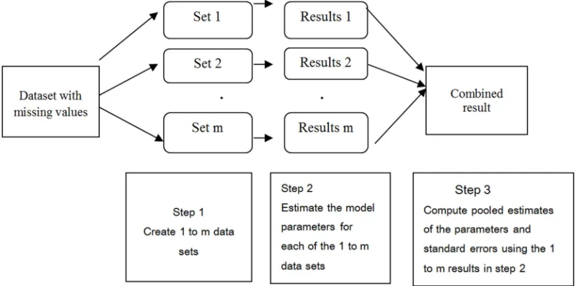
Figure 1. Multiple Imputation Steps.
The procedure takes into account the uncertainty associated with the missing values, this method is applicable when data are missing at random. Unlike the ad hoc methods, multiple imputation combines both classical and Bayesian statistical techniques using suitable models to create "
imputed datasets which takes into account the uncertainties associated with the missing values ([34]). The usefulness of multiple imputation in accounting for missing values has been documented in many research works ([35]; [3]; [28]; [1]; [7]). The imputation model should be specified accurately so that the degree of uncertainty about the missing data will be adequately reflected and, data relationships and associations are preserved ([3]; [30]; [22]). When using multiple imputation, we assume that observations are missing at random (MAR) to make it possible to ignore the process that causes the missing data ([30]). Under MAR, the multiple imputation approach retains the advantages of maximum likelihood (ML) method and allows the uncertainty caused by the imputation to be incorporated into the complete-data analysis ([22]). Multiple imputation consists of three basic steps outlined as; i) imputation step to create m complete datasets using the chosen imputation model, ii) analysing each of the m-imputed dataset separately, and iii) combining the m results into a single estimate using the Rubin’s rule. These steps are presented in Figure 1. Multiple imputation (MI) allows for the use of complete-data analysis methods and incorporates random errors to account for the uncertainties associated with the missing values ([34]). Multiple imputation performs better by minimizing the standard errors and increasing the efficiency of estimates as compared to the single imputation methods and, can be implemented using any model on any data without requiring
specialized software. Random seed should be set to ensure reproducibility of results. There are several number of multiple imputation (MI)) approaches which have been proposed for dealing with missing data problems. [13], combine the advantages of kernel estimators where kernel-based sampling weights were developed to create imputations, and the popular doubly robust methods developed to handle the misspecification of the outcome model. They used these two strategies to develop a kernel-based doubly robust MI method which is more robust than parametric alternatives against the misspecification of the outcome model.
2.3. Pooling the m Parameter Estimates for Inference
Each of the m imputed dataset is analysed using complete-data analysis method specified for the research under identical conditions. To draw inference about the population, all the " estimates of the parameters being considered are combined into single values ([34]; [38]) thereby yielding;
1 ˆ
m
i i
Q Q
m
= =
∑
(6)where EF is the pooled parameter estimate and EG 1 ⋯ "
is the parameter estimate for the () imputed complete
dataset. The combined standard error using Rubin’s rules ([34]) is slightly more complex as there are two components that make up the total error. Let EG be the estimate of a scalar quantity of interest obtained from the imputed dataset
The overall standard error for the imputation process is the sum of within and between variances, where; the within-imputation variance is represented by
1 1 m
i i
U U
m =
=
∑
(7)and the between-imputation variance by
(
)
21
1 ˆ
1
m
i i
B Q Q
m =
= −
−
∑
(8)and the total variance is then calculated by adding the within and between variances ([21]) as follows:
1 1
T U B
m
= + +
(9)
The overall standard error and confidence intervals associated with the parameters of interest can be estimated in the normal way while the degrees of freedom is given as;
(
)
(
)
2
1 1
1
mU
df m
m B
= − +
+
(10)
The rate of missing data is used to determine the number of data sets to impute, [34] and [3] suggest that for practical purposes, small number " ≤ 5 of repeated imputations is adequate to produce estimates which give valid inferences. Some scholars however recommend that m ranges from 20 to 100 or more as using large number of imputed datasets improves the stability of results more especially when estimating small size effect ([21]; [2]). The relative efficiency of the estimates could however be evaluated using
K1 +MNOP (11)
where m is the number of imputed datasets and Q the proportion of missing values in the data set. Inference based on multiple imputation are more efficient than those based on the ad hoc methods which either discard cases with missing values or impute once without taking into account the uncertainties associated with the missing values ([28]).
3. Simulation and Results
Four simulated data on disk polishing was used to illustrate some methods for handling missing data. The performance of the different methods were compared using the following datasets;
a complete data set (to serve as control).
b part of the complete data were set missing at 5% and 35% and analyzed using listwise deletion.
c use mean substitution to analyze the two datasets in (ii).
d use multiple imputation to analyze the two datasets in (ii).
The usefulness of some of the methods of handling missing data is demonstrated using the simulated data on the time it takes to polish a disk based on the thickness of the disk (mm), diameter of the disk (cm) and amount of hardener (grams) added to the cast. Fifty nine (59) sets of measurements with 5% and 35% of values set missing randomly were used. Regression analysis was used on the complete data to model the time it takes to polish a disk to serve as a control. Three methods of handling missing data; Listwise Deletion (LD), Mean Substitution (MS) and Multiple Imputation (MI) were studied and compared with the control. The parameter estimates together with their standard errors are presented in Table 2.
Table 2. Parameter Estimates under Different Imputation Methods.
Missing Rate
Imputation Methods
Control LD MS MI
0% 5% 35% 5% 35% 5% 35%
Intercept -5.129 -5.95 -17.461 -8.228 -15.034 -6.698 -20.656
(6.78) (7.48) (15.31) (7.74) (9.36) (7.2) (8.53)
Diameter 3.539 3.754 4.215 3.599 3.345 3.612 4.126
(0.51) (0.53) (0.99) (0.55) (0.64) (0.53) (0.53)
Thickness -0.56 -0.92 -2.658 -0.577 3.08 -0.705 -2.21
(1.59) (1.59) (4.07) (1.67) (3.14) (1.64) (2.45)
Hardener 2.417 0.889 9.747 4.183 6.538 3.034 11.43
(3.05) (3.59) (4.42) (3.42) (3.59) (3.27) (3.14)
4. Discussion
With LD, any case with at least one missing value is omitted, hence the residual standard error was calculated on 44 degrees of freedom as 11 observations were deleted with 5% of the observations missing giving estimates comparable with the complete case. With 35% missingness rate, 49 of the observations were deleted thereby giving biased estimates.
to enable the choice of the best method to use.
5. Conclusion
The methods discussed are all useful in handling missing data, however their application depends on how much of the data are missing and what causes the data to be missing. This paper provide researchers, more especially those with little or no understanding of statistics with guidance on how to handle missing data efficiently. The detail description of the missing data mechanisms, pattern of missing values and why the data got missing will adequately equip the researcher to make informed decision in the design of the research and the choice of the method to use. In all, the choice of method for handling missing data should be guided by the need to preserve the essential characteristics of the data, maintain the representativeness of the analyzed data, provide valid statistical inference (control Type I error), maximize the statistical power of the test (minimize Type II error), and avoid bias. However it is recommended that researchers should put in place measures that minimise the occurrence of missing values in the first instance to enhance the quality and validity of inferences obtained from incomplete data. Consultation with professionals and experts in survey design and experimentation could be the first step in overcoming the challenges of missing data.
References
[1] Acock, A. C. (2005). Working with missing values. Journal of Marriage and Family. 67; 1012-1028.
[2] Ader, H. J. {2008). Missing data. In Ader, H. J. & Mellenbergh, G. J. (Eds). Advising on research Methods: A consultant’s companion. (pp. 305-332). Huizen, The Netherlands: Johannes van Kessel Publishing.
[3] Allison, P. D. (2000). Multiple imputation for missing data: A cautionary tale. Sociological Methods & Research, 28 (3); 301 – 309.
[4] Allison, P. D. (2003). Missing data techniques for structural equation modeling. Journal of Abnormal Psychology. 112 (4); 545-557.
[5] Beasley, T. M. (1988). Comments on the analysis of data with missing values. Multiple Linear Regression Viewpoints. 25, 40-44.
[6] Blackwell, M., Honaker, J. and King, G (2011). Multiple Over imputation: A Unified Approach to Measurement Error and Missing Data.
[7] Bolotin, A. (2010). Anew method of multiple imputation for completely (or almost completely) missing data. Proceeding MACMESE'10 Proceedings of the 2th WSEASinternational conference on Mathematical and computational methods in science and engineering.
[8] Burke, S. (1998). Missing values, outliers, robust statistics & non-parametric methods. LC•GC Europe Online Supplement.
Scientific Data Management. 2 (2), 19–24.
[9] Carpenter, J. R. (2010). Statistical modeling with missing data using multiple Imputation. www. missingdata. org.uk. [10] Carpenter, J. R. and Kenward, M. G. (2008). Missing data in
randomized controlled trials-a practical guide. Birmingham: National Health Service Coordinating Centre for Research Methodology, www.missingdata.org.uk.
[11] Carter, R. L. (2006). Solutions for missing data in structural equation modeling. Research & Practice in Assessment. 1 (1); 20-27.
[12] Chen, S. (2014) "Imputation of missing values using quantile regression". Unpublished Graduate Theses and Dissertations. Iowa State University. http://lib.dr.iastate.edu/etd/13924. [13] Chiu-Hsieh, H., He, Y., Li, Y., Long, Q. and Friese, R. (2016).
Doubly robust multiple imputation using kernel-based techniques. Biom J. 58(3): 588-606.
[14] Davey, A. and Savla, J. (2010). Statistical power analysis with missing data: A structural equation modeling approach. NY: Routledge; 47-65.
[15] Enders, C. K. (2006). A primer on the use of modern missing-data methods in psychosomatic medicine research.
Psychosomatic Medicine, 68;.427-436.
[16] Fisher, A. and Waclawski, A. (2009). A survey of techniques for identifying and handling outliers and missing values in time series data. 29th International Symposium on Forecasting. Hong Kong. ww.forecasters.org/isf.
[17] Foster, P. J., Mami, M. A. and Bala, A. M. (2009). On treatment of the multivariate missing data. Research Report No. 13, Probability and Statistics Group, School of Mathematics. The University of Manchester.
[18] Glas, C. A. W. and Pimentel, J. L. (2008). Modeling Non-ignorable Missing Data in Speeded Tests. Educational and Psychological Measurement 68 (6), 907-922.
[19] Graham, J. W. (2009). Missing data analysis: Making it work in the real world. Annual Review of Psychology, 60; 549-576.
[20] Graham, J. W., Cumsille, P. E. and Elek-Fisk, E. (2003). Methods for handling missing data. In J. A. Schinka & W. F. Velicer (Eds.), Research Methods in Psychology (pp. 87-114).
Handbook of Psychology, New York: John Wiley & Sons. [21] Graham, J. W., Olchowski, A. E., and Gilreath, T. D.
(2007). How many imputations are really needed: Some practical clarifications of multiple imputation theory.
Prevention Science, 8, 206-213.
[22] He, Y. (2010). Missing data analysis: Getting to the heart of the matter. Journal of the American Heart Association.
3; 98-105.
[23] Horton, N. J. and Kleinman, K. P. (2007). Much ado about nothing: A comparison of missing data methods and software to fit incomplete data regression models. The American Statistician, 61(1), 89-90.
[24] Kang, H. (2013). The prevention and handling of the missing data. Korean J Anesthesiol.; 64(5): 402–406. [25] Kenward, M. (2007). Missing Data with MLwiN: An
[26] Kim, J. O. and Curry, J. (1977). The treatment of missing data in multivariate analysis. Sociological Methods & Research, 6 (2); 215-240.
[27] Litttle, R. J. A. (1988). A test of missing completely at random data with missing values. Journal of the America Statistical Association. 83 (404); 1198-1202.
[28] Little, R. J. A. and Rubin, D. B. (2002). Statistical analysis with missing data, (2nded.). New York: John Wiley & Sons. [29] Okafor, R. (1982). Bias due to logistic non-response in sample
survey. (Unpublished Ph. D. Thesis Submitted to the Department of Statistics, Harvard University. Cambridge, Massachusetts).
[30] Patrcian, A. P. (2002). Focus on research methods: Multiple imputation for missing data. Research in Nursing and Health, 25, 76-84.
[31] Peng, C. Y., Harwell, M. R., Liou, S. M., & Ehman, L. H. (2006). Advances in missing data methods and implications for educational research. In S. S. Sawilowsky (Ed.), Real Data Analysis. (pp. 31-78). New York.
[32] Pigott, T. D. (2001). A review of methods for missing data.
Educational Research and Evaluation, 7 (4); 353-383. [33] Rubin, D. B. (1976). Inference and missing data. Biometrika,
63;581–592.
[34] Rubin, D. B. (1987). Multiple imputation for non-response in Surveys. New York: Wiley.
[35] Schafer, J. L. (1997). Analysis of incomplete multivariate data, New York: Chapman and Hall.
[36] Schafer, J. L. and Graham, J. W. (2002). Missing data: Our
view of the state of the art. Psychological Methods, 7(2); 147-177.
[37] Schwartz, T., Chen, NY Q. and Duan, NY N. (2011). Studying missing data patterns using a SAS® Macro. Statistics and Data Analysis, SAS Global Forum. Paper 339.
[38] Song, Q., Shepperd, M., Cartwright M. and Twala, B. (2005), A New imputation method for small software project data sets.
[39] Stratton, I. M., and Aldington, S. J. (2007). Missing data means lost opportunities. Journal of Clinical Research Best Practices. 3, (5).
[40] Stuart, E. A., Azur, M., Frangakis, C. and Leaf, P. (2009). Multiple imputation with large data set: A case study of the children’s mental health initiative. American Journal of Epidemiology, 169 (9); 1133-1139.
[41] Swetha, S. (2016). An Integral Study on Missing Value Data Imputation. International Journal of Engineering Sciences & Research Technology. 5(2). 356-365.
[42] Todorov, V., Templ, M. and Filzmoser, P. (2011). Detection of multivariate outliers in business survey data with incomplete information. Advance Data Analyses and Classification. 5; 37-56.
[43] vonHippel, P. T. (2013). Should a normal imputation model be modified to impute skewed variables? Sociological Methods and Research, 42 (1); 105-138.