Determination of One Dimensional Temperature Distribution in Metallic Bar Using Green’S Function Method

Published online October 30, 2013 (http://www.sciencepublishinggroup.com/j/ajam) doi: 10.11648/j.ajam.20130104.14

Determination of one dimensional temperature

distribution in metallic bar using green’s function method

Virginia Mwelu Kitetu

1

, Thomas Onyango

1

, Jackson Kioko Kwanza

2

,

Nicholas Muthama Mutua

3

1_{Department of Mathematics and Computer Science, Faculty of Science, the Catholic University of Eastern Africa, Nairobi, Kenya} 2_{Department of Pure & Applied Mathematics, Jomo Kenyatta University of Agriculture & Technology, Nairobi, Kenya}

3_{Department of Mathematics and Informatics, School of Science and Informatics, Taita Taveta University College, Voi, Kenya}

Email address:

[email protected](V. M. Kitetu), [email protected](T. Onyango), [email protected](J. K. Kwanza), [email protected](N. Muthama)

To cite this article:

Virginia Mwelu Kitetu, Thomas Onyango, Jackson Kioko Kwanza, Nicholas Muthama Mutua. Determination of One Dimensional Temperature Distribution in Metallic Bar Using Green’S Function Method.American Journal of Applied Mathematics.

Vol. 1, No. 4, 2013, pp. 55-70. doi: 10.11648/j.ajam.20130104.14

Abstract:

The present study focuses on determination of temperature distribution in one dimensional bar using Green’s

function method. The Green’s Function is obtained using separation of variables, variation formulation principles and Heaviside functions. The Boundary Integral Equation is obtained using the fundamental solution, Divergence theorem, Green Identities, Dirac delta properties and integration by parts. The solution of heat equation given by the Green’s Function and the boundary integral equation has satisfied the uniqueness, regularity and stability of heat equation. The uniqueness, regularity and stability have been proved using smooth properties of class k function, Lyapunov function and 2

L Norm. The BEM implementation is performed using FORTRAN 95 software. Solutions to the test problems are presented and time dependence results are in agreement with computed analytical solutions.

Keywords:

Green’s Function, Heaviside Function, Separation of Variables, Integration by Parts, Lyapunov Function

1. General Introduction

1.1. General Description and Terminologies

1.1.1. Temperature

Temperature is the measure of coldness or hotness of a body. In a qualitative manner, we can describe the temperature of an object as that which determines the sensation of warmth or coldness felt from contact with it. A convenient operational definition of temperature is that it is a measure of the average translational kinetic energy associated with the disordered microscopic motion of atoms and molecules. The International System of Units (SI) for temperature is Kelvin (K). Other units are degree Celsius, Fahrenheit, Rankine, Delisle, Newton, Reaumur and Romer.

1.1.2. Heat Flux

Temperature and heat flow are two important quantities in the problems of heat conduction. Temperature at any point in the solid is completely defined by its numerical value because it is a scalar quantity, whereas heat flow is defined by its value and direction. The basic law which gives the

relationship between the heat flow and temperature gradient is by French mathematician Jean Baptiste Joseph Fourier. He focused on a stationary, homogeneous, isotropic solid (materials in which thermal conductivity is independent of direction).The law is of the form

T

k

q

=

−

∇

(1)

1.1.3. Modes of Heat Transfer

Heat is energy transferred from a high temperature system to lower temperature system. Its International System of units (SI) is Joule (J). Heat transfer is a discipline of thermal engineering concerned with generation, use, conversion and exchange of thermal energy and heat between physical systems. There are three modes of heat transfer namely conduction, convection and radiation.

conductors of heat. Non-conductors (insulators) include plastic, clay, wood and paper. The rate of heat flux (rate of heat transfer per unit area) in a solid object is proportional to the temperature gradient. The Fourier law is

dx

dT

kA

q

_x

=

−

(2)

Convection: refers to the heat transfer that occurs between a surface and fluid when they are at different temperatures. Convection heat transfer mode is comprised of two mechanisms such energy transfer due to random molecular motion (diffusion) and energy transferred by the bulk or macroscopic motion of the fluid (advection).

Convection leads to the fact that good insulators (like air) can transfer heat efficiently -as long as the air is allowed to move freely. Trapped air, as between panes of a double window, cannot transfer heat well because it cannot mix with air of a different temperature. Convection heat transfer may be classified according to the nature of the flow. Forced convection takes place when the flow is caused by an external agent such as fan, pump or atmospheric winds. Natural convection is caused by buoyancy forces due to density differences caused by temperature variations in the fluid. Free convection flow field is self-sustained flow driven by the presence of a temperature gradient. Mixed convection is experienced when natural and forced convection occurs together. Newton’s law of cooling is

(

−

∞

)

=

h

T

T

q

''

_s (3)

Radiation is the transfer of heat in form of waves through space (vacuum). Heat is carried by electromotive waves from one medium to another. Radiation takes place between two surfaces by emission and later absorption. Stefan Boltzmann’s equation is given by

(

4

)

1 4 2

T

T

ASe

q

=

−

(4)

1.2. Literature Review

Ozisik (1968) studied the physical significance of Green’s function in heat conduction. He presented the general expressions for the solution of inhomogeneous transient heat conduction problems with energy generation, inhomogeneous boundary condition, and a given initial condition, in terms of Green’s function for one, two and three dimensional problems of finite and semi-infinite regions.

Chang and Tsou (1977) in their book entitled “Heat conduction in Anisotropic Medium Homogeneous in cylindrical Regions-Unsteady State” discussed about the analytical solution of heat conduction in an anisotropic medium that is homogeneous in circular cylindrical co-ordinates. They considered boundary conditions of Dirichlet, Neumann and mixed types of solid cylinder and hollow cylinder of finite and infinite lengths.

Cannon and John (1984) in their book entitled “The one

dimensional Heat Equation” researched on some Green's function solutions in 1D.A variety of elementary Green's function solutions in one-dimension are recorded here. In some of these, the spatial domain is the entire real line

(-∞, ∞). In others, it is the semi-infinite interval (0, ∞) with either Neumann or Dirichlet boundary conditions.

Beck (1984) derived the Greens function solution for the linear, transient heat conduction equation in the form that included five kinds of boundary conditions and also demonstrated the conditions under which it was permissible to use the product property of one dimensional Green’s functions.

Greenberg (1986) in his book “Application of Greens Function in Science and Engineering” analyzed some application of Green’s function to solve conduction heat transfer, acoustic gravitational potential and vibration problems.

James and Jeffrey (1987) applied Green’s function to solve heat conduction equation in three dimensions obtaining an integral equation for temperature in terms of the initial and boundary values of the temperature and flux.

Copper and Jeffery (1998) studied the flow of heat in one dimension through a small thin rod. They used the derivation of the heat equation, and Mat lab’s to model the motion and showed graphical solutions. They used two methods to solve the rate of heat flow through an object. The first method was derived from the properties of the object. The second method was derived by measuring the rate of heat flow through the boundaries of the object.

Eduardo (2001) formulated a table of Green’s Function that enable us to derive transient conduction solutions for rectangular co-ordinates system and also provided a numbering system that enables efficient cataloging and locating of Green’s Function. The Green’s Function was obtained using Eigen functions expressions.

Praprotnik et al. (2002) discussed the numerical solution of the two dimensional Heat Equation. An approximation to the solution function is calculated at discrete spatial mesh points, proceeding in discrete time steps. The starting values are given by an initial value condition. They explained how to transform the differential equation into a finite difference equation which can be used to compute the approximate solution.

Vijun (2004) analyzed piezoelectric parallel Bimorph using BEM. He concluded that BEM solves these problems faster than the other methods. He also predicted temperature distribution using combined BEM and FEM for heat transfer in fuel cell.

sources and showed that for discrete sources Green’s function determined by method of images yielded analytical solutions.

Misawo F. (2011) researched on a solution of one dimensional transient Heat transfer problem using Boundary Element Method (BEM).She modeled the flow of heat from a hot cylindrical metal billet to a liquid of uniform temperature. The cylinder was considered to have many thin slabs across the volume which when heated summed up to form the whole volume.

Duhamel’s method relates the solution of boundary-value problems of heat conduction with time-dependent boundary conditions and heat sources to the solution of similar problem and heat sources by means of simple relation .Duhamel’s method is a useful tool for obtaining the solution of a problem with time-dependent boundary conditions and heat sources whenever the solution of a similar problem with time- independent boundary conditions and heat source is available. A proof of Duhamel’s method is given by Bartels and Churchil (1942) for a building condition of first kind. This method is used to solve heat conduction in semi-infinite solid, semi-infinite rectangular strip and long solid cylinder.

1.3. Research Objectives

The purpose of this work is to determine one dimensional temperature distribution on a metallic bar using the Green’s Integral Method. The specific objectives are:

1. To determine a general Green’s function solution equation applicable to the solution of heat transfer by conduction.

2. To apply the Green’s function solution equation considered to determine boundary integral equation for temperature distribution.

3. To determine temperature and flux profile using BEM.

1.4. Significance of the Study

In recent years, applied mathematics has developed a strong interest in the science of heat and mass transfer. This is mainly due to its many applications in engineering, astrophysics, and geophysics and power generation, among others

Heat transfer is of great significance to branches of science and engineering. Heat transfer is very important to engineers who have to understand and control the flow of heat through the use of thermal insulation, heat exchangers such as boilers, heaters, radiators, refrigerators and other devices. Thermal insulators are materials specifically designed to reduce the flow of heat by limiting conduction, convection or both. Radiant barriers are materials which reflect radiation and therefore reduce the flow of heat from radiation sources. A heat exchanger is a device built for efficient heat transfer from one fluid to another, whether the fluid is separated by a solid wall so that they never mix, or fluids are directly contacted.

Heat exchangers are widely used in refrigerators, air conditioning, space heating, power production, and chemical processing, the radiator in car, in which the hot

radiator fluid is cooled by the flow of air over the radiator surface. The modern Electric and electronic plants require efficient dissipation of thermal losses, hence a thorough heat transfer analysis is important for proper seizing for fuel elements in the nuclear reactor cores to minimize burn out.

The performance of an aircraft also depends upon the ease with which the structure and the engine can be cooled. The utilization of solar energy which is widely used in refrigerators, air conditioning space heating, power production and chemical production readily available requires a thorough knowledge of heat transfer for proper design of the solar collectors and associated equipments.

2. Governing Equations

Heat transfer problems can be described by set of equations namely: the heat equation, Heaviside function, Dirac-Delta Function, the Divergence theorem, Green Identities and Laplace equation

2.1. The Heat equation

Consider a heated solid body with constant thermal conductivity, k, with solution domain

0

<

x

<

1

, the conservation law for heat transfer in the body in one dimension is given the heat equation

(5)

for k > 0. This equation which is also known as the diffusion equation can be solved by imposing boundary conditions. The most common four boundary conditions applicable to it are:

Dirichlet boundary condition, which specify the dependent variable u(x,t) at each point of the boundary, I = (0, l) of the region within which solution is required, mathematically we can represent Dirichlet Boundary conditions as:

, , ,

Neumann boundary condition, which specify the flux of the dependent variable u(x,t) at each point of the boundary, I=(0,l) of the region within which solution is required, mathematically can be represented as:

, , ,

Robin boundary condition or mixed boundary condition is a combination of Dirichlet and Neumann boundary conditions. It specifies the flux and the function u(x,t) at each point of the boundary I = (0, l) of the region within which the solution is required, mathematically is represented as:

, , ,

variable u(x,t) in periodic shape. Mathematically is represented as:

1, ,

2.2. Heaviside Function

It is unit step function, named after the electrical engineer Oliver Heaviside, it is defined as:

(

)







>

<

=

−

1

1

1

0

x

if

x

if

a

x

H

(6)

Heaviside function and Dirac-Delta function is related by the following property

( ) ( )

x

dx

x

dH

₌

_δ

(7)

2.3. Dirac-Delta Function

Sometimes is called the Unit Impulse Function. It models phenomena of an impulse nature such as action of heat flow over a very short time interval or over a very small region. Situation like this occurs in mechanics especially when a force concentrated at a point caused by deformation on solid surface, impulse forces in rigid body dynamics, point mass in gravitational field theory, point charges and multipoles in electrostatics. And more important for this study is as point heat sources and pulses in theory of heat conduction. The Green’s Function is the response of a differential equation, and the Dirac Delta function describes the impulse.

The Dirac Delta Function

δ

( )

x

is zero when x≠0, and infinite at x=0 in such a way that the area under the function is unity i.e.:

0 0 (8a)

∞ 0 (8b)

1

∞

∞ (8c)

2.3.1. Physical Interpretation of Dirac Delta and Fundamental Solution

The Dirac delta function is used in physics to represent a point source. A continuous temperature distribution in 3-dimensional space is described by a temperature density, typically denoted

ρ

( )

x

. The total temperature of the distribution is given by integrating the temperature density all over space:

(9)

Now suppose that I have a single point charge, q, at position

x

'

. The charge density of a point charge should be zero everywhere except at

x

=

x

'

, since there is no charge anywhere except at this point. On the other hand, at

x

'

, we have a finite charge in an infinitely small volume, so the density should be infinite there.

Finally, it must satisfy,

Q

=

∫

d

3

x

ρ

( )

x

since q is the total charge. These requirements are uniquely satisfied by

( )

x

=

q

δ

(

x

−

x

'

)

ρ

(Temperature density of a point charge q at

x

'

)

One would have similar expressions for the (mass) density of a point mass m.

The function

δ

( )

x

is essentially a bookkeeping device; it is a singular function which is zero everywhere except at the position x = 0 (the origin of the coordinate system) where it is infinite. Some basic properties of Dirac delta are:

•

Q

=

∫

d

3

x

ρ

( )

x

•

ρ

( )

x

=

q

δ

(

x

−

x

'

)

•

d

3

( ) ( )

x

δ

x

=

1

•

( )

( )

x

dxf

( ) (

x

x

a

) ( )

f

a

a

ax

=

∫

−

=

∞

∞ −

δ

δ

δ

1

•

∫

( ) (

−

'

)

=

1

∞

∞ −

x

x

x

dxf

δ

•

δ

(

x

−

x

'

) (

=

δ

x

'

−

x

)

2.4. The Divergence Theorem

This theorem is also known as Gauss Theorem. It states that the flux of a smooth vector field

F

through a closed boundary

µ

=

∂

Ω

equal to integral of its divergence. Mathematical statement is

∫

∫

F

n

ˆ

dx

=

_Ω

div

F

d

Ω

µ (10)

where

n

ˆ

is the outward normal to surface µ and is enclosed Ω region.

Gauss theorem is very important in vectorial calculus. If

F

is continuous vector field and its components have continuous partial derivatives in Ω, then

∫∫

∫∫∫

∇

⋅

Ω

=

Ω

F

d

µ

F

n

ˆ

d

µ

(11)

2.5. Green’s Identities

Take vector function

F

=

V

∇

U

where U and V are arbitrary scalar fields, defined in Ω. Then

U

V

U

V

F

=

∇

+

∇

⋅

∇

⋅

∇

2 ₍₁₂₎

n

V

U

n

U

V

n

F

∂

∂

=

⋅

∇

=

⋅

ˆ

ˆ

(13a)

n

U

V

n

U

V

n

F

∂

∂

=

⋅

∇

=

⋅

ˆ

ˆ

(13b)

yields Green’s first identity:

(

)

_µ

d

µ

n

U

V

d

U

V

U

V

∫∫

∫∫∫

∇

+

∇

⋅

∇

Ω

=

∂

_∂

Ω 2 (14)

If

F

=

U

∇

V

_{, substituting this in divergence equation}

(10) results into:

(

)

_µ

d

µ

n

V

U

d

V

U

V

V

∫∫

∫∫∫

∇

+

∇

⋅

∇

Ω

=

∂

_∂

Ω 2 (15)

Subtracting equation (15) from (14) gives Green’s Theorem (Green’s second identity) i.e.

(

)

∫∫

∫∫∫













∂

∂

−

∂

∂

=

Ω

∇

−

∇

Ω µ

_n

U

V

n

V

U

d

U

V

V

U

2 2 (16)

2.6. Fundamental Solution of the Problem

A fundamental solution for a linear partial differential operator L is a formulation in the language of distribution theory of a Green's function. In terms of the Dirac delta function δ(x), a fundamental solution G is the solution of the inhomogeneous equation.

( )

x

LG

=

δ

(17)

The usefulness of the Green function is evident once you make the following realization. Any distribution of source (i.e. charge density for instance) can be written as a sum, or integral in the continuous case, of point sources. Therefore, if we know how the system reacts to a point source, then we should be able to determine how it reacts to any distribution of source, since we can sum up all the contributions. It is absolutely critical here that the differential operator is linear. The fundamental solution is an approximation which is used in boundary integral equation.

Consider heat transfer equation (5), a modeled for heat transfer through a metallic bar, is obtained using method of separation of variables see equation 19, under prescribed initial conditions u(x,0)=f(x), Boundary conditions are

±∞

→

→

as

x

U

0

(18)

( )

x

t

F

( ) ( )

t

G

x

U

,

=

(19)

Substituting equation (19) into heat equation (5) results into ,

F

_T

G

=

kFG

_xx, dividing this equation by kFG gives

t

Con

G

G

kF

F

_{t xx}

tan

=

=

, where the constant is

−

D

2

Solving

D

2

kF

F

_t

−

=

i.e.

F

_t

+

kD

2

F

=

0

results into:

( )

kDt

e

c

t

F

=

₁ − 2 (20)

where

c

1 _{is constant.}

Solving,

D

2

G

G

_xx

−

=

i.e.

0

2

=

+

D

G

G

_xx , yields:

( )

x

c

ei

c

e

x

G

=

₂ Dx

+

₃ −iD (21)

Where

c

₂ and

c

₃ are constants.

Substituting equations (21) and 20 into (19) gives:

( )

kDt

(

iDx iDx

)

e

c

e

c

e

c

t

x

U

,

=

₂ − 2 ₂

_

₃ − (22)

Substituting the boundary conditions U(∞,t)=U(-∞,t)=0 into (22) results into:

The physical significance of boundary condition is that using Dirac delta function,

δ

( )

x

=

0

if

x

≠

0

, the integration on interval is zero .

( )

x

t

Ae

(

iDx

kD

t

)

U

_,

=

−

2 ₍₂₃₎

Integrating (23) with respect to D on (-∞, ∞) results into:

( )

( )

(

iDx kDt

)

e

D

A

t

x

U

,

− 2

∞

∞ −

∫

=

( )

x

t

A

( )

D

e

(

)

dD

U

,

iDx−kD2t

∞

∞ −

∫

=

(24)

Substituting the initial condition, U(x,0)=f(x) into (24) gives

( )

x

A

( )

D

e

DdD

f

∫

ix

∞

∞ −

=

(25)

Then using Fourier transform theorem, equation (25) becomes:

( )

( )

'

'

2

1

_'

dx

e

x

f

D

A

−ixD

∞

∞ −

∫

=

π

(26)

Inserting (26) into equation (24) yields

( )

( 2)

( )

'

1

, ' '

2

iDx kD t _{ix D}

U x t e f x e dx dD

π ∞ ∞ − ₋ −∞ −∞     =      

∫

∫

(27)

Rearranging equation (27), we obtain:

( )

( )

_{( )}

_'

_'

2

1

,

t

e

' 2

dD

f

x

dx

x

U

∫

∫

ix x D kDt

∞ ∞ − ∞ ∞ − − −













=

π

(28a)

( )

x

,

t

G

(

x

,

x

'

,

t

) ( )

f

x

'

dx

'

U

∫

∞

∞ −

=

(28b)

(

_x

_x

_t

)

_e

( )

_dD

G

∫

ix x D kDt

∞

∞ −

− −

=

_' 2

2

1

,

'

,

π

(29a)

or

(

)

1

{

(

)

(

)

}

2

, ', cos ' sin '

2

kD t

G x x t x x D i x x D e dD

π

∞

−

−∞

=

_∫

− + − (29b)

The second integrand in equation (29b) is zero since sine is an odd function.

(

x

x

t

)

{

(

x

x

)

De

}

dD

G

∫

kDt

∞ ∞ − −

−

=

2

'

cos

2

1

,

'

,

π

(29c)

Integrating equation (29c) using integration

rule,

∫

∞

∞ −

−

−

₌

a

b ax

e

a

bxdx

e

4 2 2

cos

π

Where our

a

=

kt

,

b

=

(

x

−

x

'

)

, then equation (29c) becomes the Green’s function for heat equation

(

)

( kt)

x x

e

kt

t

x

x

G

4 '2

4

1

,

'

,

− −

=

π

(30)

Substituting equation (30) into equation (28b) results into:

( )

( )

( )

'

'

4

1

,

4 '

dx

x

f

e

kt

t

x

U

kt x x− − ∞ ∞ −

∫

=

π

(31a)

When

f

( ) (

x

=

δ

x

−

x

'

)

and using Dirac delta function,

(

−

)

=

1

∫

∞ ∞ −

dx

a

x

δ

, see equation (8c)

Equation (31a) reduces to, fundamental solution of one dimension, heat equation given by

( )

(

)

(

)

kt

x

x

e

kt

t

x

x

G

t

x

U

π

π

4

'

4

1

,

'

,

,

2

−

−

=

=

(31b)

Using Heaviside function, H, which is introduced to emphasize the fact that the fundamental solution is zero if

o

t

t

≤

equation (31b) reduces into:

(

)

(

₍

)

₎

((t to))

x x e o o o

t

t

k

t

t

H

t

x

t

x

U

− − −

−

−

=

4 '2

4

,

'

,

,

π

(31c)

Where

t

−

t

_o it the time period.

2.7. The Boundary Integral Equation

We are using Greens theorem equation (16), taking V=G(x,t), when we first rewrite the heat equation using the

Del operator, ₂

2

x

∂

∂

=

∆

.

( )

x

t

k

U

( )

x

t

U

_t

,

=

∆

,

(32)

Where

x

≤

x

'

∈

Ω

and

0

<

t

≤

t

_o.

Given that the Green’s function G(x,t), satisfies properties of heat and Green’s functions, namely:

G

k

G

_t

=

−

∆

(33a)

( )

x

t

=

on

∂

Ω

G

,

0

(33b)

( ) (

x

,

t

x

x

'

)

G

_o

=

δ

−

(33c)

Multiplying the heat equation (32) by Green’s function,

(

x

x

t

)

G

,

'

,

and integrating over the volume and over time integral we get:

(

)

(

)

0 0

o o

t t

t

G U dxdt G k U dxdt

Ω ⋅ = Ω ⋅ ∆

∫ ∫∫

∫ ∫∫

(34)

Integrating the LHS of (34) by parts by letting u=G and

!

Therefore, " and v=U, then the LHS of (34) becomes

(

)

(

)

0

(

)

0 0 | o o o t t t t t

G U dxdt G U dx U G dxdt

Ω Ω

Ω

⋅ = ⋅ − ⋅

∫ ∫∫

∫∫

∫ ∫∫

(35a)

Using equation (33a), to simplify equation (35), we obtain

(

)

(

)

0

(

)

0 0 | o o o t t t t

G U dxdt G U dx kU G dxdt

Ω Ω

Ω

⋅ = ⋅ + ∆

∫ ∫∫

∫∫

∫ ∫∫

(35b)

Integrating RHS of (35b) twice by parts by taking u=G and

2 2 U dV U n ∂ = ∆ =

∂ then simplify we have,

(

)

( )

( )

( )

0 0 0

0

o o o

o

t t t

t

U

G k U dxdt kU Gdxdt kG dS x dt

n

G

kU dS x dt

n Ω Ω ∂Ω ∂Ω ∂ ⋅ ∆ = ∆ + ∂ ∂ − ∂

∫ ∫∫

∫∫∫

∫ ∫

∫ ∫

(36a)

(

)

( )

( )

0 0 0

o o o

t t t

G

G k U dxdt kU Gdxdt kU dS x dt

n

Ω Ω

∂Ω

∂

⋅ ∆ = ∆ −

∂

∫ ∫∫

∫∫∫

∫ ∫

(36b)

Equating (35b) and (36b) gives,

( )

(

)

( )

( )

0 0

0

0

0 0

0

. |o

t t

t

t

GU dx kU G dxdt kU Gdxdt

G kU dS x dt

n

Ω Ω Ω

∂Ω

+ ∆ = ∆

∂ −

∂

∫∫

∫∫∫

∫∫∫

∫ ∫

(37)

Equation (37) reduces into:

( )

0

( )

0 0

. |o t

t G

GU dx kU dS x dt

n

Ω

∂Ω

∂ =−

∂

∫∫

∫ ∫

(38)

Writing the Left Hand Side of (38) as

( )

. |0

(

'

)

(

, ';0,0

)

o t

GU dx U x x dx f G x x t dx

Ω

Ω Ω

= ⋅ − − ⋅

∫∫

∫∫

∫∫

(39a)

Which by property of delta function we get,

( )

. |0

( )

',0

(

, ';0,0

)

o t

GU dx U x t f G x x t dx

Ω

Ω

= − ⋅

∫∫

∫∫

(39b)

Inserting (39b) into (39a) we get,

( )

(

)

0

( )

0 0

0

', , ';0,

t

n

G

U x t f G x x t dx kU dS x dt

n

Ω

∂

∂

− ⋅ =−

∂

∫∫

∫∫

(40a)

Making

U

(

x

'

,

t

₀

)

the subject of the formula gives heat

function, (BIE) in the solution domain which will then be discritised using BEM.

( )

(

)

0

( )

0 0

0

', , ';0,

t

n

G

U x t f G x x t dx kU dS x dt

n

Ω

∂

∂

= ⋅ −

∂

∫∫

∫∫

(40b)

2.8. Statement of the Problem

People who work under high temperature conditions need to know the temperature distribution in those areas after a certain period of time. They should be equipped with knowledge on temperature distribution from high temperature to low temperature and insulation methods to minimize heat lose.

Heat distribution in a metallic rod has been determined using non linear methods and found not accurate. We are using numerical method, Green function method to improve the accuracy through the use of boundary integral method assuming the metallic bar has the following dimensions.

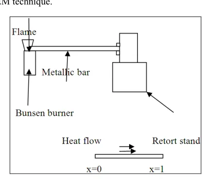
Consider heat flow from boundary x=0 to x=1, with specified Dirichlet and Robin boundary conditions,

unknown temperatures are obtained numerically using BEM technique.

Figure 1.1. Geometrical Configuration of the research problem

2.9. Assumption of the Study

i. The metallic bar is of unit length. ii.Temperature is discretely distributed.

iii.Thermal conductivity of the metallic bar is one.

3. Methodology

The Green’s function integral method is selected because the solution is always in the form of an integral and can be seen as a recasting of boundary value problem into integral form. The Green’s function method is useful if the Green’s function is known and if the integral expressions can be evaluated. Overcoming these limitations offers Green’s function several advantages for solution of linear heat conduction problems. Even if the integral has to be evaluated numerically this is generally more accurate than numerical solution such as finite differences especially for discrete sources. The advantages of the Green’s function method s are the following;

1.It is flexible and powerful. For a given geometry it can be used as building block to the temperature resulting from: space-variable initial conditions, time and space variable boundary conditions and time and space variable generation.

2.It has a systematic solution procedure. For a given Geometry, the Green’s function for a particular type of boundary conditions can be determined once .This can be used for any type of source, and the solution for Temperature can be written immediately in the form of integrals. The systematic procedure saves time and reduces the possibility of error, which is particularly important for two and three dimensional geometrics. 3.It has minimal computation labor when compared to

purely numerical finite difference or finite element methods. It has much better accuracy than finite difference techniques.

infinite series solution for heat conduction problems driven by non-homogeneous boundary conditions problem exhibit slow convergences, requiring a very large number of terms to obtain accurate numerical values. For some of these problems, an alternative formulation of the Green’s function solution reduces the number of required series terms.

3.1. Method of Solution

In this study for simplicity we reduce the heat equation to one dimension, unsteady case which is then written using Greens function method which uses variation formulation principles. The fundamental solution of heat equation G(x,x`,t) is obtained using method analytical approach. The heat equation is then discritised using BEM when in cooperating the Greens function. The boundary conditions are then prescribed by describing the temperature distribution on the specified boundaries of the solution domain.

3.2. Numerical Discretisation of the BIE

This technique is necessary because it transforms the Boundary Integral Equation into a linear system of equations that can be solved by a numerical approach. In choosing the interval points it is important that any corner of the boundary µ and also any point where a prescribed boundary condition changes are included. This ensures each of the intervals of the boundary is smooth, so that the normal is well defined at each nodal point, and a single boundary condition applies within each interval. The interval of the boundary is symmetrically distributed about any of the axes of symmetry, and such axes intersect with the boundary at interval points rather than at nodal points.

By the classical BEM methodology, Brebbia et al (1984), and using the fundamental solution for the time dependent heat equation in one dimension given by equation (31c) the heat equation can be transformed into the following boundary integral equation,

( )

(

)

(

)

(

)

1

2

0 0 1

0 , , ', , , ', , , ', s s U G

U x t G x x t t U x x t ds

n n

UG x t x t ds

∂ ∂   = _ − _ ∂ ∂   +

∫

∫

(40c)

The integral over

S

₃ vanishes due to the Heaviside function in expression (31c).

The discretisation of the BIE (40c) is performed using the following steps:

The boundaries

S

₁and

S

₂ are discretised into a series of small boundary elements.

{ }

{ }

1 1

1

0 (0,

0

( ,

N

f j j

j

S t t− t

=

 

= × =

∪

×  (41a)

{ }

{ }

2 1

1

1 (0,

1

( ,

N

f j j

j

S t t − t

=

 

= × =

∪

×  (41b)

T he boundary

S

₃ is discretised in a series of small cells

[ ]

{ }

0

{

]

{ }

3

1

0,1 0 , 0

N

k k

k

S x x

=

= ×

∪

× (41c)

Over each boundary element the temperature U and the

flux

n

U

∂

∂

are assumed to be constant and take their values at

the midpoint,

2

~

j 1 j

j

t

t

t

=

−

+

(42) i.e.

( )

0,

( )

0, j o

U t =U j U jfor

t

∈

(

t

_j−1

,

t

_j

)

(43)

( )

1,

( )

1, j 1j

U t =U j =U for

t

∈

(

t

j−1

,

t

j

)

(44)

( )

( )

0 0, 0, ' j j U j U t U n n ∂ ∂ =

∂ ∂ for

t

∈

(

t

j−1

,

t

j

)

(45)

( )

( )

1 1, 1, ' j j U j U t U n n ∂ ∂ =

∂ ∂ for

t

∈

(

t

j−1

,

t

j

)

(46)

Also, over each cell the temperature U is assumed to be constant and takes its value at the midpoint,

2

~

k 1 k

k

x

x

x

=

−

+

(47)

( )

(

)

0

, 0 k, 0 k

U x =U xɶ =U _for

(

]

k k

x

x

x

∈

₋₁

,

(48)

With the approximations (43) to (48) and k=1, the boundary

integral equation (40b) is discretised as:

( )

(

)

(

)

(

)

(

)

(

)

1 1 1 1 0 1 ' '

0 0 0 0 0 0

1 1

0 0 0 1 0 0

1 0 1 1

0'

0 1

, , ,0, , ,1,

, ,1, , ,1,

, ,0, ',0

j j j j j j j j k k t t N N j j

j t j t

t t

N N

j j

j t j t

x N

k

j x

U x t U G x t t dt U G x t t dt

G G

U x t t dt U x t t dt

n n

U G x t x dt

− − − − − = = = = = = + ∂ ∂ − − ∂ ∂  + _

∑

∫

∑

∫

∑

∫

∑

∫

∑

∫

For

( )

x t, ∈

[ ]

0,1×

(

0,1

]

(49)

Where #$ and # represent the outward normal at the

boundaries x=0 and x=1 respectively.

discretised boundary integral form of the time-dependent heat equation in one dimension as:

( )

( )

( )

( )

( )

( )

0

0 ' 1 ' 0 ' 1 '

0 0 0 1

1

0 1

, , , , ,

,

N

j j j j j j j j

j N

k k

k

U x t C U x t C U x t D U x t D U x t

E x t U

=

=



=  + − −

+

∑

∑

(50)

Where coefficients are given by

(

)

(

)

(

(

)

)

1 1

2 '

0 0 0

0 0

' 1

, , ',

4 2

j j

j j

t t

x j

t t

x x

C G x t x t dt e dt

t t t t

π

− −

− −

= =

− −

∫

∫

(51)

(

)

( )

(

( )

)

1 1

2 '

0 0

' 0 0

' 1

, , ', ( '

4 2

j j

j j

t t

x j

x

t t

x x G

D x t x t dt x x e dt

n π _{t t} t t

− −

− − ∂

= = −

∂ − −

∫

∫

(52)

( )

(

)

(

₍

)

₎

1 1

2 0

0

' 1

, , ', ,0

4 2

kj k

k k

x x

k

x x

x x

E x k G x x t dt e dt

t t t

π

− −

− −

= =

−

∫

∫

(53)

If the boundary integral equation (40b) has these approximations applied at every node on the boundary

S

₁

then the following set of linear algebraic equations is obtained.

( )

0

( )

0 ' ' 1 ' ' 0 ' 1 ' 0

0 1 0 1

1 1

' ' 0

N N

x x x x

ij j ij j ij j ij j ik k

j k

C U C U D x U C U E x U

= =

 _{+ − −} _{+ =}



∑

∑

(54),

1, %

&&&&&_, '_{( )0,1*}

Where the influence matrices +$ ,, + ,, -$ , and - , are defined by

+_./$ , ₊ /

,

0, ̌. , +./

,

+_/, 1, ̌. (55) 1.2 ' 12 ', ̌. (56)

Also, on applying the initial condition (48) at the cell nodes (32, 0) for 1, %&&&&&&$ , then the values !2$ are

determined, namely,!0 !

4

, 0 32 ), 1, %$

&&&&&& ₍₅₇₎

Recasting together equations results in a system of equations which in a generic form can be written as

5. 7 8 (58)

Where X is a known

4

N

×

4

N

square matrix which includes the influence matrices+$, + , -$, - and E given by expression (4c)-(44), 7 is a vector of 4N unknowns which contains the unknowns !$., !., !$.' 9# !'.

recasted as 7. !$. for 1, %&&&&&

3.3. Method of Solution of the Problem

This section presents method of solution to heat transfer

problem, in particular, heat flow through a metallic bar (along its length) which is analyzed by modeling transfer through a geometry (0,1)x (0,1).Rearranging equation (54) according to the specified boundary conditions, BEM FORTRAN 95 code for the computation of unknown values is developed. To validate the numerical implementation, solutions to the test problems are presented. The graphs are drawn with the help of G-sharp software.

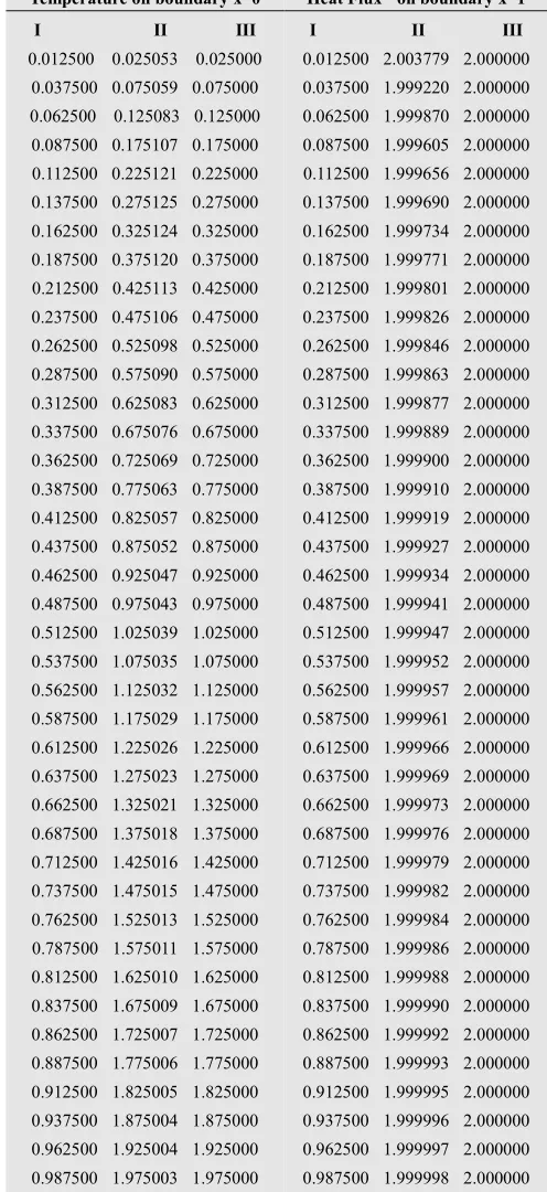
3.3.1. Problem 1: Approximated Values on the Boundaries

Consider heat equation ! ! which is modeled by heat transfer through a metallic bar with analytical solution given by

! , = 2+2 (59) Initial conditions U(x,t)=0,

Boundary conditions are

U(0,t)=2t (60)

U(1,t)=1+2t (61)

! =2, ! =2, ! =! k=1 (62) Assuming heat lost on both ends and insulation on the sides, BEM code is implemented considering boundary discretisation of 20 Nodes. The results obtained are illustrated in the graphs below.

3.4. Existence and Regularity of Heat Equation Solution Using Initial Data, U(x,0)=f(x)

The equation for conduction of heat in one dimension for a homogeneous body has the form

ut=kuxx

The Cauchy problem for this equation consists in specifying U(0, x)= f(x), where f (x) is an arbitrary function.

Existence and uniqueness theorem is the tool which makes it possible for us to conclude that there exists only one solution to a first order differential equation which satisfies a given initial condition.

Theorem 1 The heat equation with bounded continuous initial data f(x) has a solution for

−∞ < x < ∞ and t > 0, defined by equation (31b), and u(x, t) satisfies u(x, 0) = f(x) in the sense that

lim $= ,

Actually, you can put in functions f which aren’t continuous or bounded; all we really need is that f doesn’t grow too fast (faster than

2

x

e

) or be so discontinuous that the integral doesn’t make sense.

3.4.1. Speed of Propagation

The heat equation has interesting qualitative features such as speed of propagation.

small interval (a, b). Because the exponential function is never zero, the integral typically won’t be zero, even for small t and x arbitrarily far from (a, b). More generally, the initial condition f affect the solution u(x, t) for all x, no matter how small t is. The heat propagates with infinite speed.

3.4.2. Smoothing Properties Using Class K Functions

In a mathematical analysis a differentiability class is a classification of functions according to the properties of their derivatives. Higher order differentiability classes correspond to the existence of more derivatives. Functions that have derivatives of all orders are called smooth.

Consider an open set on the real line and a function f defined on that set with real values. Let k be a non-negative integer. The function f is said to be of class

C

k if the derivatives

f

'

,

f

''

,...,

f

( )k exist and are continuous (the continuity is automatic for all the derivatives except for

f

( )k . The function f is said to be of class

C

_∞, or smooth, if it has derivatives of all orders. The function f is said to be of class

C

_∞, or analytic if f is smooth and if it equals its Taylor series expansion around any point in its domain.

In general, the classes Ck can be defined by declaring C0 to be the set of all continuous functions and declaring Ck for any positive integer k to be the set of all differentiable functions whose derivative is in Ck−1. In particular, Ck is contained in Ck−1 for every k, and there are examples to

show that this containment is strict.

C

∞is the intersection

of the sets Ck as k varies over the non-negative integers. First, recall that a function is said to be

C

∞if it is infinitely differentiable i.e. we can differentiate as many times as we like and the derivatives never develop corners or discontinuities. For heat equation solution, the function

( ) kt

x x

e

kt

4 '2

2

1

− −

π

is such a function, with respect to all

variables. Also, for any t > 0 this function decays to zero very rapidly away from

x

=

x

'

. As a result, we can differentiate both sides of equation (31) with respect to x as many times as we like, by slipping the x derivative inside the integral to find

( )

1

(

'

)

2

( )

, ' '

4 2

n n

x x

U x t e f x dx

kt

x πkt π

∞

−∞

 _{− −} 

∂ _{=  }

 

∂

∫

_{ } (63)

The integral always converges (if, e.g., f is bounded). In short, no matter what the nature of f (discontinuous, for example) the solution U(x, t) will be

C

∞in x, for any time t > 0; the initial data is instantly smoothed out.

3.4.3. Uniqueness and Stability of Heat Equation Solution Using Lyapunov Function

In the theory of ODEs, Lyapunov functions are scalar functions that may be used to prove the stability of equilibrium of an ODE. For many classes of ODEs, the existence of Lyapunov functions is a necessary and sufficient condition for stability.

A Lyapunov function is a function that takes positive values everywhere except at the equilibrium in question, and decreases along every trajectory of the ODE. The main advantage of Lyapunov function is that the actual solution (whether analytical or numerical) of the ODE is not required. This can be extended to PDES heat equation which is convertible to ODE via separation of variable.

If U(x, t) satisfies the heat equation, define the quantity

( )

1 2

( )

, ,

2

E x t U x t dx

∞

−∞

=

_∫

(64)

where

E

( )

x

,

t

is a Lyapunov function, (assuming the integral is finite) similar to the energy for the wave equation. It’s not clear if

E

( )

t

above is physically any kind of “energy”, but it can be used to prove uniqueness and stability for the heat equation.

It’s easy to compute

( ) ( )

, t ,

dE

U x t U x t dx

dt

∞

−∞

=

∫

(65)

provided U and

U

_tdecay fast enough at infinity which we’ll assume. Replace

U

_t in the integral with

U

_xx

(since

U

_t

−

U

_xx

=

0

) to find,

( ) ( )

, xx ,

dE

U x t U x t dx

dt

∞

−∞

=

_∫

(66)

Now integrating by parts (take an x derivative off of

U

_xx,

put it on u) to find

( )

( ) ( )

( )

lim lim 2

, , , ,

x x x x

dE

U x t U x t U x t U x t dx

dt

∞

→∞ →∞

−∞

= − −

_∫

(67)

We will assume that U limits to zero as |x| → ∞, in fact, impose this as a requirement. Assuming

U

_x stays bounded,

we can drop the endpoint limits in

dt

dE

above (alternatively,

we could assume

U

_x limits to zero and U stays bounded). We obtain

2

( , )

dE

U x t dx

dt

∞

−∞

It’s obvious thatdE 0

dt ≤ , so

E

( )

t

is a non-increasing

(and probably decreasing) function of t. Thus, for example,

( )

0

>

0

≤

E

for

t

E

of course

E

( )

t

is simply the

L

2 norm of the function

U

( )

x

,

t

, as a function of x at some fixed time t, and we’ve shown that this quantity cannot increase in size over time. Here’s a bit of notation: we use

( )

.,

t

₂

U

to mean the

L

2norm of U as a function of x for a fixed value of t. With this notation we can formally state the following Lemma:

Lemma 1 Suppose that

U

( )

x

,

t

satisfies the heat equation for −∞ < x < ∞ and t > 0 with initial data U(x, 0) = f(x). Then

( )

2 2

.,

t

f

U

≤

we can wipe out uniqueness and stability at the same time. Consider two solutions

1

U

and

U

₂ to the heat equation, with initial data

f

₁ and

f

₂. Form the function

U

=

U

₁

−

U

₂, which has initial data

f

₁

−

f

₂ . Apply Lemma 1 to U and you immediately obtain

Theorem 2 If

U

₁and

U

₂ are solutions to the heat equation for −∞ < x < ∞ and t > 0 with initial data

U

₁

( )

x

,

0

=

f

₁

( )

x

and

U

₂

( )

x

,

0

=

f

₂

( )

x

, and both

1

U

and

U

₂ decay to zero in x for all

t

>

0

, then

( )

( )

2 2 1 2 2

1

.,

t

U

.,

t

f

f

U

−

≤

−

.

To prove uniqueness take

f

₁

=

f

₂ to conclude that at all times t > 0 we have

U

₁

−

U

₁

=

0

Or

(

( )

( )

)

2

1 , 1 , 0

U x t U x t dx

∞

−∞

− =

∫

This for

U

₁

−

U

₁

=

0

, so

U

₁

( )

x

,

t

=

U

₁

( )

x

,

t

for all

x

and

t

.

3.4.4. Uniqueness and Stability of Heat Equation Solution Using 2

L Norm

For the wave equation we measure how close two functions f and g are on some interval

a

[

<

x

<

b

]

(either a or b can be ±∞) using the supremum norm

( ) ( )

x

g

x

f

SUP

g

f

−

_∞

=

_a<x<b

−

(we can also talk about the size or norm of a single function, as

f

_∞

=

SUP

_a<x<b

f

( )

x

. There’s another common way to measure the distance between two functions on an interval

(a, b), namely

( ) ( )

(

)

2

2

b

a

f −g =

∫

f x −g x dx (69)

We can also measure the norm of a function with

( )

(

)

∫

=

b

a

dx

x

f

f

2

2 (69)

The latter quantity is called the

L

2 norm, so the distance between two functions can be measured as the

L

2norm of their difference. It’s easy to see that if

0

2

=

f

then f

must be the zero function, and

0

2

=

−

g

f

implies

f

=

g

.

The norm

L

2 is very much like the usual Pythagorean norm for vectors from linear algebra (or just Calc I), which for a vector

X

=<

x

₁

,

x

₂

,...,

x

_n

>

is defined as

( )

2 2

1

n j j

X x

=

 

=  



∑

 (70)

4. Results and Discussion

Problem 1

When temperatures are specified on boundary x=0 and x=1 respectively the results at various levels of time are computed and illustrated in the graphs below for 20 Nodes.

Figure 1a: Approximated and analytical flux on boundary x=0

Problem 2

When fluxes are specified on both boundaries the results at various levels of time ate computed and illustrated below.

Figure 2a: Approximated and analytical temperatures on the boundary x=0

Figure 2b: Approximated and analytical temperatures on the boundary x=1

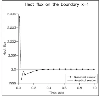
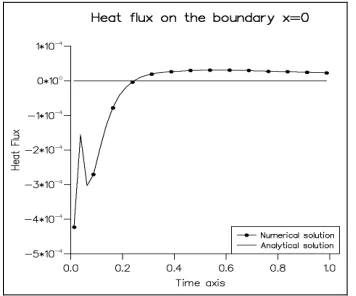
Problem 3

When flux and temperatures are specified on either boundary the results at various levels of time ate computed and illustrated below.

Figure 3a: Approximated and analytical flux on the boundary x=0

Figure 3b: Approximated and analytical temperatures on the boundary x=1

Figure 4a: Approximated and analytical temperatures on the boundary x=0