1. Introduction
Project scheduling is about the determination of the starting time of the activities. In addition to activities, the material ordering, delivering time are important factors in every project. These three variables including activities start time, ordering, and delivering time of materials are considered in the Project Logistic Problem (PLP). In fact, PLP is critical because of its role in the project-planning phase when the activities start time is affected by the time of material delivery. In other words, in the real world, there is no any project in which when its activities want to start, all of its required materials are already prepared. However, PLP is not enough to schedule the project correctly. For example, consider the project in which the activities are done by labors that have to move between each activity and where the materials are gathered (warehouses). These trips between the places each activity is done and the warehouses make the project scheduling more complex.
Corresponding author
E-mail address: [email protected] DOI: 10.22105/jarie.2019.170649.1079
Simultaneous Solution of Material Procurement Scheduling
A
nd
Material Allocation to Warehouse Using Simulated Annealing
Nima Moradi , Shahram Shadrokh
Department of Industrial Engineering, Sharif University of Technology, Tehran, Iran.
A B S T R A C T P A P E R I N F O
One of the classes of the project schedule is the Material Procurement Scheduling (MPS) problem, which is considered besides the material allocation to warehouse (MAW) problem recently. In the literature, the Simultaneous Solution of MPS-MAW is investigated by considering one warehouse and unlimited capacity of the warehouses most of the times. In this paper, we propose the propositional and mathematical model of the simultaneous MPS-MAW with multiple warehouses and the limited capacity at the whole of the horizon planning for each warehouse. The proposed model aims to obtain the best ordering point, selection of the best suppliers, the best activity start, and the fair material distribution to the warehouses as possible by the given objective function. The proposed model is NP-hard, so a metaheuristic namely simulated annealing is proposed to reach the acceptable but not optimal solutions in a short time. Also, to overcome the complexity of the model, the encoding of the decision variables have been done by adding the auxiliary variable. Comparing the solutions of the small problems with the exact methods shows the validation of the proposed SA. Also, the design of experiments shows the significance of the model and each SA parameters. Finally, by the optimum values of the SA parameters, the large problems have been solved at acceptable times.
Chronicle:
Received: 03 December 2018 Revised: 01 March 2019
Accepted: 12 March 2019
Keywords: Material Procurement
Schedule.
Material Allocation to Warehouse. Simulated Annealing. Design of Experiments.
Journal of Applied Research on Industrial
Engineering
In each project, in addition to the Material Procurement Scheduling (MPS), the Material Allocation to the Warehouse (MAW) must be considered. In fact, if we only consider MPS, the solution to the problem will be a local minimum. On the other hand, if we just solve MAW, the solution will be a local minimum one, because, in MAW, the allocation and material transportation costs are considered which are insufficient to model the objective function of the real projects. Therefore, the consideration of both MPS and MAW is necessary in order to reach the global optimum solution through the modeling with more reality. In this paper, we aim to solve MPS and MAW simultaneously, so that the cost of material ordering from different suppliers and costs related to MAW are minimized by the optimum determination of the material ordering, delivering and activities start times and the quantities of the materials allocation to the warehouses.
2. Literature Review
PLP has been investigated by many researchers. One of the papers which have solved PLP with integrating the procurement and construction processes is [1] in which the ordering time and quantity of the materials were determined by considering the stochastic construction process. Also, the optimum ordering and activities start times were obtained by considering the lag between the ordering time and delivering time of the materials through the progress curve of the delivery and construction process in order to avoid lateness. The lag between the ordering time and material delivery time was considered as a stochastic parameter. Finally, by determination of the sufficient stock of materials through the mathematical formulas, the project is protected from being late by the optimum scheduling of the ordering time and construction process start time.
The article [2] investigated the construction resource planning and scheduling by simulation and analytical techniques. In other words, the near-optimum distribution of the different resources such as manpower, equipment, space, and material in the life cycle of the project is the main purpose of this paper. To solve the problem, an intelligent scheduling system (ISS) was proposed in which the duration, cost and Net Present Value (NPV) of the project had been minimized. Although the distribution of resources is the important factor, material allocation is not considered in this paper.
By [3], the procurement scheduling for complex projects had been investigated with the fuzzy environment. The activities duration and lead times are fuzzy. Their fuzzy mathematical programming is able to determine the optimum ordering time with considering the shortage and holding costs. While the ordering point is important, but the activities start time must be considered in the model.
In the paper [4], two separated problems – MPS and Project Scheduling Problem (PSP)–are integrated under the different suppliers. For this integrated problem, they proposed the mixed-integer programming model with holding, ordering, purchasing and activities related costs as an objective function without consideration of the capacity of the warehouses. Their solution technique was an enhanced Genetic Algorithm (GA), which was able to solve the problem when its size was going to arise in a reasonable time.
warehouse’s capacity is not mentioned, while this is an important factor when the warehouse space is limited like the real projects.
In the paper [6], the MPS and PSP are solved simultaneously by the hybrid SA and GA. Their proposed model has two costs of ordering and holding. The decision variables are the start time of the activities, the ordering time and quantity, and the inventory level for only one warehouse. Also, the project duration is limited by the deadline and there is no supplier in the model. The results show that the proposed hybrid SA-GA is more efficient than the exact methods when the problem size is rising. The previous article had been developed by the paper [7] with consideration of the multi-mode activities and quantity discount policy. Their mixed integer programming model consists of three objective functions called the project duration minimization, maximization of the robustness of the project and minimization of the total costs including ordering, holding, procurement, and resources employment. The project is constrained by deadline and resource availability, while the capacity of the warehouse is not considered. Then, the proposed model is solved by multi-objective problems solution methods like NSGAII, SPEAII, MOPSO, and MOEAD. The results show that the NSGAII is better than the other method in most of the metrics.
The paper [8] has investigated the integrated planning of project scheduling and material procurement with consideration of the environmental impacts. The proposed mixed integer model aims to determine the optimum value of the activity start time, ordering time, and quantity while considering the constraints of the resources availability, ordering quantity and environmental impacts with two objective functions. The solution techniques are NSGA-II and MOMBO. The results show the better efficiency of the MOMBO when the instances are getting larger. Moreover, by [9] the Project Scheduling and Material Ordering (PSMO) problem had been solved by two multi-objective metaheuristic algorithms called NSGA-II and MOPSO. Their contributions were considering the economic, environmental, and social concerns in the objective functions and using the data of the real case study in Iran.
As the papers related to our topic have been reviewed, it can be seen that the papers modeled the MPS and PSP by just one warehouse, so that not considering the multiple warehouses is a gap in the literature. Also, the above-mentioned articles just consider the one related cost to warehouses or inventories as a holding cost of the resources ; this is the second gap. In fact, the costs related to the warehouses can be developed by determination of which materials allocate to which warehouse in order to minimize the material travel distance on the project site, because when the materials come to the work site, at first, they are assigned to the proper warehouses and then, they are used by the related activities; this is the third gap. In addition, by considering multiple warehouses, in addition to their capacities, which is less considered in the literature even for one warehouse, the fair distribution of the materials to the warehouses can be added to the objective function. Therefore, the contributions of this paper can be listed below:
Considering the multiple warehouses on the project site.
Considering the material allocation to warehouses problem besides the MPS. Considering the fair distribution of the materials to the warehouses.
In the next Section, the problem is stated in which the MPS and MAW are investigated with more details and the details of the decision variables, and objective functions are mentioned too. In the third part, the propositional and the mathematical models are proposed. In the fourth part, the solution technique is introduced and its functions are explained. In the fifth part, we have the results and discussions about the outputs. Finally, in the last part, the conclusions and recommendations for future studies are proposed.
3. Problem Statement
The problem of this paper can be seen as two separated parts called before delivery and after delivery. In the first part, before the materials deliver to the activities, the ordering and delivering time and also, selection of the supplier are determined. After that, in the second part, when the materials reach the site, the selection of the warehouses which the materials allocate to them and the activities start time are determined. In other words, not only the activities schedule is affected by the ordering and delivering times, but also the material allocation to the warehouses is determined by the activities location. So, the project costs are not limited to ordering or holding costs. In fact, the material transportation costs are included too by the solution of MAW. In the following, the assumptions or the propositional model and mathematical model are proposed.
3.2 Problem Modeling
In this section, the propositional model or the structured assumptions are proposed. This propositional model is the structured form of the assumptions which we can understand the whole problem and see its strong points or weak points by them.
3.1.1 The propositional model
In the site modeling, the location of each warehouse is predetermined and dimensionless. The shape of each material is dimensionless.
Each material for each activity is ordered only one time with the predetermined quantity. The material transportation cost per unit is predetermined.
The quantity of material transportation is equal to the material ordering quantity. The lead time for each material by each supplier is deterministic.
The unit of time is discrete.
The activity start time must be bigger than the delivering time of the materials. Each material must be ordered from only one supplier.
Each warehouse has a limited capacity. Each activity location is predetermined.
The distance between each activity location and each warehouse is predetermined. Each material for each activity must be allocated to only one warehouse.
The requirement material for each activity is deterministic and predetermined. There is no discounted ordering.
Each activity can be started between its earliest start time and latest start time.
The material can leave the warehouse when its related activity wants to start, otherwise, the material will stay in the warehouse.
The activities are finish-to-start with zero lag, non-preemptive, deterministic duration, with one mode and without cash flow.
There is a penalty when the materials distribution to the warehouses is not fair.
Now by the above-mentioned propositional model, the mathematical model is available. 3.1.2 The mathematical model
The notations, indices, sets, parameters, and decision variables are defined below:
Indices
j=1,…,N Index of activities.
m=1,…,M Index of materials.
s=1,…,S Index of suppliers.
t=0,…,H Index of time.
l=1,…,L Index of warehouses.
Sets
𝐽𝑡 The set of activities, which can be started at t.
𝑂𝑡 The set of activities, which their requirement material can be ordered at t.
𝐵𝑗 The set of activities preceding j.
Parameters
N Number of activities.
M Number of materials.
L Number of warehouses.
S Number of suppliers.
H The horizon of planning.
𝐺𝑚𝑠 The cost of ordering material m form supplier s.
ℎ𝑚 The holding cost of material m in each warehouse.
𝑅𝑗𝑚 The requirement material m for activity j.
𝐿𝑚 Lead time of material m for each supplier.
𝐹𝑙 The maximum capacity of the warehouse l.
𝑑𝑗 The duration of activity j.
𝑒𝑗 The earliest start time of the activity j. 𝑙𝑗 The latest start time of the activity j.
𝐶𝑚 The transportation cost per unit of the material m.
𝐷𝑙𝑗 The distance between the warehouse l and the location of the activity j. P The amount of the penalty of the unfair material distribution per unit.
Decision variables
𝛾𝑚𝑗𝑠𝑡 Equals to 1 if the material m is ordered from supplier s for the activity j at the time t and 0, otherwise.
𝑦𝑚𝑗𝑙𝑡 Equals to 1 if the material m that is ordered for activity j is allocated to warehouse l at the time t and 0, otherwise.
𝐼̅ The mean of the amounts of 𝐼𝑙.
In the following, the mathematical model is proposed below:
(1)
𝑀𝑖𝑛 𝑍 = (∑(𝐼𝑙− 𝐼̅)2)/(𝐿 − 1) × 𝑃 𝐿 𝑙=1 , + ∑ ∑ ∑ ∑ 𝐺𝑚𝑠× 𝛾𝑚𝑗𝑠𝑡 𝑒𝑗−𝐿𝑚 𝑡=0 𝑆 𝑠=1 𝑁 𝑗=1 𝑀
𝑚=1 ,
+ ∑ ∑ ∑ ∑ 𝑅𝑗𝑚× 𝐷𝑙𝑗× 𝐶𝑚× 𝑦𝑚𝑗𝑙𝑡 𝐻−1 𝑡=𝐿𝑚 𝐿 𝑙=1 𝑁 𝑗=1 𝑀
𝑚=1 ,
(2)
𝑖 ∈ 𝐵𝑗
𝑗 = 1,2, … , 𝑁 𝑠. 𝑡. ∑ 𝑡 ∗ 𝑋𝑖𝑡 𝑙𝑖 𝑡=𝑒𝑖 + 𝑑𝑖≤∑ 𝑡 ∗ 𝑋𝑗𝑡 , 𝑙𝑗 𝑡=𝑒𝑗 (3)
𝑋10= 1,
(4)
𝑗 = 1,2, … , 𝑁 ∑ 𝑋𝑗𝑡 = 1
𝑙𝑗
𝑡=𝑒𝑗 ,
(5)
𝑙 = 1,2, … , 𝐿 𝐼𝑙= ∑ ∑ ∑ 𝑦𝑚𝑗𝑙𝑡∗ 𝑅𝑗𝑚 , 𝑒𝑗 𝑡=𝐿𝑚 𝑁 𝑗=1 𝑀 𝑚=1 (6)
𝑙 = 1,2, … , 𝐿 𝐼𝑙≤𝐹𝑙,
(7)
𝑚 = 1,2, … , 𝑀 𝑗 = 1,2, … , 𝑁
∑ ∑ 𝛾𝑚𝑗𝑠𝑡
𝑒𝑗−𝐿𝑚
𝑡=0 𝑆
𝑠=1 = 1,
(8)
𝑚 = 1,2, … , 𝑀 𝑗 = 1,2, … , 𝑁
∑ ∑ 𝑦𝑚𝑗𝑙𝑡
𝑒𝑗
𝑡=𝐿𝑚 𝐿
𝑙=1 = 1,
(9)
𝑚 = 1,2, … , 𝑀 𝑗 = 1,2, … , 𝑁
∑ ∑ 𝑡 ∗ 𝛾𝑚𝑗𝑠𝑡
𝑒𝑗−𝐿𝑚
𝑡=0 𝑆
𝑠=1 = ∑ ∑ 𝑡 ∗ 𝑦𝑚𝑗𝑙𝑡
𝑒𝑗
𝑡=𝐿𝑚 𝐿
𝑙=1 − 𝐿𝑚,
(10)
𝑚 = 1,2, … , 𝑀 𝑗 = 1,2, … , 𝑁
∑ ∑ 𝑡 ∗ 𝛾𝑚𝑗𝑠𝑡
𝑒𝑗−𝐿𝑚
𝑡=0 𝑆
𝑠=1 ≤ ∑ 𝑡 ∗ 𝑥𝑗𝑡
𝑙𝑗 𝑡=𝑒𝑗 − 𝐿𝑚, (11) 𝐼̅ = (∑ 𝐼𝑙 𝐿 𝑙=1 )/𝐿, (12)
𝑚 = 1,2, … , 𝑀 𝑙 = 1,2, … . , 𝐿 𝑗 = 1,2, … . , 𝑁 𝑡 = 0,1, … , 𝐻 𝑋𝑗𝑡 {0,1} , 𝑦𝑚𝑗𝑙𝑡{0,1}, 𝛾𝑚𝑗𝑠𝑡{0,1}, 𝐼𝑙≥ 0 𝐼𝑛𝑡𝑒𝑔𝑒𝑟.
earliest and latest start time. Constraint (5) calculates the overall inventory of each warehouse of the cycle time of the project. Constraint (6) limits the overall inventory of each warehouse with the aim of controlling the fair material distribution. By constraint (7), each material of each activity must be ordered at interval time between 0 and its activity earliest start time (𝑒𝑗) minus its material lead time
(𝐿𝑚) just one time and from one supplier. By constraint (8), each material of each activity must be
allocated to only one warehouse at interval time between (𝐿𝑚) and its activity earliest start time (𝑒𝑗) just
one time. By constraint (9), after 𝐿𝑚 time unit, ordered material must be delivered to its related activities. By constraint (10), after 𝐿𝑚 time unit, ordered material can be allocated to its related activities. Constraint (11) calculated the mean of the amounts of 𝐼𝑙. At last, by constraint (12), the type
of the decision variables of the model is determined. From the complexity theory viewpoint, the above-mentioned mathematical model is in the class of NP-hard problems.
Proof
Premise: Based on the literature the Multi-Dimensional Travel Salesman Problem (MTSP) is in the class of NP-complete problems.
Argument: If in the above-mentioned model the material allocation section is removed, the MPS remains. Furthermore, by MTSP, we want to find a path with the minimum sum of the distances that each salesman meets every city just one time and returns to its first city. If in MTSP instead of the cities, we consider the project operations such as ordering, delivering, allocating, and processing, and also, we consider each material as each salesman, MTSP can be reducible to MPS problem. So, MPS problem is at least as hard as MTSP.
Conclusion: By the premise (i) and argument (ii), therefore, MPS problem or our mathematical model is in the class of NP-hard problems.
Our proposed mathematical model is NP-hard. As a result, we cannot reach the optimal solution if the size of the problem increases. So, in the following, a metaheuristic algorithm is proposed to reach an acceptable but not optimal solution when the problem size rises.
4. Simulated Annealing for MPS-MAW
In this section, a simulated annealing optimization algorithm is proposed. Our SA is not modified basically, but its functions of generating the neighborhood solution are adapted to the decision variables of the problem, which it is described in the following. SA was introduced by [10] for the first time. Its function is influenced by the natural phenomenon in which the molecular structure of the metals is getting organized when it gets cold gradually. Three references [11-13] are sufficient to understand the concept and how to implement the SA. SA is a single-solution based algorithm basically. Hence, SA improves only one solution at its iterations. This makes the SA fast; however, its performance of finding a global solution is weakened. Totally, the performance of SA of solving the combinatorial optimization problems has been proved in the literature, and this is our reason to select it as a solution technique. The pseudo code of the proposed SA is presented below that is coded by C++ programming.
a) Inputs b) Cooling starts
Generate an initial solution (𝑠 = 𝑠0);
Set initial temperature (𝑇0= 𝑇𝑚𝑎𝑥); i=0;
While (𝑇𝑖> 𝑇𝑚𝑖𝑛) do
{ t=0;
{
Generate the neighborhood solution by function M (𝑠́); Calculate the (∆𝐸 = 𝑓(𝑠) − 𝑓(𝑠́));
If ((∆𝐸 ≤ 0) then 𝑠 = 𝑠́ Else
{
𝑟𝑎𝑛 =a random number between 0 and 1; If (𝑟𝑎𝑛 ≥ 𝑒−∆𝐸⁄𝑇𝑖) then 𝑠 = 𝑠́
Else continue; }
t++; }
Update the temperature (𝑇𝑖+1= 𝛼 ∗ 𝑇𝑖); i++;
}
c) Display the best solution.
In this pseudo code, at first step, inputs are inserted. These inputs consist of the problem parameters and SA parameters. SA parameters are described with their notation in Table 1. The notation 𝑠0 is the initial solution, which is an important factor because of its impact on the solution quality. The initial solution can be determined randomly or greedy. In this paper, we do not investigate the impact of the initial solution. The notation 𝑇𝑖 denotes the temperature of the iteration i. This temperature is cooled by the
equation 𝑇𝑖+1 = 𝛼 ∗ 𝑇𝑖 in which 𝛼 is the cooling rate. Also, if 𝛼 is valued between 0.8 and 0.99, the cooling plan will be slow and efficient [14]. The notation 𝑓(𝑠) is the objective function or fitness function of the problem. Function M generates the neighborhood solution, which is similar to mutation function of GA.
Table 1. Definition of SA parameters.
4.1 Solution Representation
The encoding of the decision variables of the problem is shown in Table 2. The problem is coded by the C++ programming and all of the decision variables are encoded by 2-dimension matrices. In order to encode the decision variables 𝑦𝑚𝑗𝑙𝑡 and 𝛾𝑚𝑗𝑠𝑡 which have the four indices, we use the auxiliary variable called 𝐴𝑚𝑗𝑡. In other words, the representation of the decision variable with four indices
increases the computational complexity. To overcome this problem, we introduce 𝐴𝑚𝑗𝑡. At first, for
each material of each activity, the ordering time is determined by the variable 𝐴𝑚𝑗𝑡. Now, for 𝛾𝑚𝑗𝑠𝑡 we just need to determine its index of supplier, because the index 𝑡 is common between 𝐴𝑚𝑗𝑡and 𝛾𝑚𝑗𝑠𝑡that
is obtained before. Also, the index 𝑡 of 𝑦𝑚𝑗𝑙𝑡 is calculated by adding amount of 𝐿𝑚to the index 𝑡 of
𝛾𝑚𝑗𝑠𝑡. Hence, the variable 𝑦𝑚𝑗𝑙𝑡 can be encoded by a 2-dimension matric in which the value of index l
Parameter Notation Definition
Maximum temperature 𝑇𝑚𝑎𝑥 Initial temperature.
Minimum temperature 𝑇𝑚𝑖𝑛 The final temperature that the algorithm stops when the 𝑇𝑖
reaches 𝑇𝑚𝑖𝑛.
Maximum iteration in each
temperature 𝑁𝑒𝑥
The temperature of the algorithm is cooled when the 𝑡 reaches 𝑁𝑒𝑥.
is determined. Variable 𝑋𝑗𝑡 is encoded by the 1-dimension matric in which each array is valued by the
discrete numbers indicate the start time of the activities.
Table2. Solution representation by C++ programming.
Solution representation Decision variables 𝑗𝑁 … 𝑗2 𝑗1 𝐴𝑚𝑗𝑡 𝑡1𝑁 … 𝑡12 𝑡11 𝑚1 … … … … … 𝑡𝑀𝑁 … 𝑡𝑀2 𝑡𝑀1 𝑚𝑀 𝑗𝑁 … 𝑗2 𝑗1 𝛾𝑚𝑗𝑠𝑡 𝑠1𝑁 … 𝑠12 𝑠11 𝑚1 … … … … … 𝑠𝑀𝑁 … 𝑠𝑀2 𝑠𝑀1 𝑚𝑀 𝑗𝑁 … 𝑗2 𝑗1 𝑦𝑚𝑗𝑙𝑡 𝑙1𝑁 … 𝑙12 𝑙11 𝑚1 … … … … … 𝑙𝑀𝑁 … 𝑙𝑀2 𝑙𝑀1 𝑚𝑀 𝑗𝑁 … … 𝑗2 𝑗1 𝑋𝑗𝑡 𝑡𝑁 … … 𝑡2 𝑡1
4.2 How to Generate Neighborhood Solutions
In this section, we define the process of function M. by function M, the code of solution is changed, as it is shown below. This function has one parameter called 𝑚𝑟 which is determines the number of arrays which have to be changed or mutated. In this paper, we call 𝑚𝑟 as mutation rate and include it in SA
parameters.
For example, for the variable 𝑦𝑚𝑗𝑙𝑡 with 𝑚𝑟 = 2, we have:
Therefore, in this section, the proposed SA is introduced. Our SA is not modified basically, but the decision variables are encoded in a simple way to decrease the computational complexity of the problem and SA is able to move towards the new solution by the mutation function. In the following, by the proposed SA, we are going to solve the problem of small and large sizes to evaluate the performance of the algorithm.
5. Computational Results
In this section, at first, we validate the proposed SA of solving the small problem by comparing its performance with the exact solution techniques, which are proposed by GAMS software. Then, the Design of Experiments (DOE) is performed in order to obtain the optimum value of SA parameters. Based on literature, DOE has been accepted as an efficient tool to conduct and analyze the experiments [15]. Finally, by the optimum SA parameters, we solve the problem with large size by the proposed SA and also, the artificial intelligence of the solution algorithm is shown by the history of convergence.
5.1 Small Problem
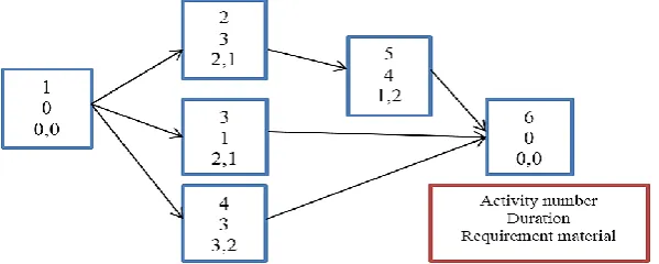
In this part, a numerical example with the size of 6 activities, 2 materials, 4 suppliers, and 2 warehouses is solved. The project network of the example with activities durations and the required material of each activity are shown in Fig. 1. The inputs of the examples with small and large sizes are not shown in this paper but they can be given if they are requested.
Fig 1. The project network of the numerical example with the small size.
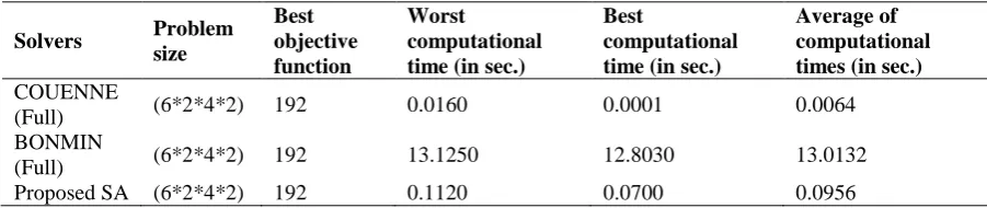
Table 3. Comparison of the results obtained by the proposed SA and exact solvers of GAMS software of the problem with the small size.
Solvers Problem size
Best objective function
Worst
computational time (in sec.)
Best
computational time (in sec.)
Average of computational times (in sec.)
COUENNE
(Full) (6*2*4*2) 192 0.0160 0.0001 0.0064
BONMIN
(Full) (6*2*4*2) 192 13.1250 12.8030 13.0132
Proposed SA (6*2*4*2) 192 0.1120 0.0700 0.0956
5.2 DOE
In this section, a DOE is organized to evaluate the relationship between each SA parameter and the computational time of the algorithm. DOE’s method is Response Surface Methodology (RSM), which its outputs is calculated by Design Expert software. The experiments are done in order to investigate the 5 SA parameters. The range of changes of each SA parameter is given in Table 4. Moreover, the DOE’s result is shown in Table 5, which shows the significance of each parameter and model. By Table 5, we can see that the parameters 𝑇𝑚𝑎𝑥, 𝛼, and 𝑁𝑒𝑥 are significant and in the other words, they have a
direct impact on the computational time of the algorithm. Also, among the dual compositions, the composition of two parameters 𝛼, and 𝑁𝑒𝑥 is distinguished significant with high certainty at the level 0.05. The significance of the other parameters and other dual compositions are given in Table 5 too. Finally, the DOE gives us the minimum value of the SA parameters in order to solve the problem in a short time as it is shown in Table 6.
Table 4. The range of changes of SA parameters in the experiments.
Now by the optimal values of SA parameters obtained by DOE process in the previous part, the large problems are getting solved in the next part that the performance of the proposed SA has been increased by the optimal values.
5.3 Large Problems
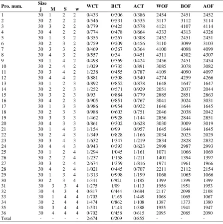
In this part, 36 examples which are available in the library of the project scheduling instances1 (PSPLIB) with the size of 30 and 60 activities, 1 to 4 materials, 2 to 4 suppliers and 2 to 4 warehouses are solved. The problems with 30 activities had been executed 5 times and the results are given in Table 7. In this table, WCT is the worst computational times among the executions, BCT is the best computational time, ACT is the average of the computational times, WOF is the worst objective function, BOF is the best objective function, and finally AOF is the average of the objective functions obtained the proposed SA of each problem. The results of Table 7 show that by increasing the problem size, the computational time has been growing which was predictable. The convergence history of the objective functions values
1 http://www.om-db.wi.tum.de/psplib/
SA parameter 𝑻𝒎𝒂𝒙 𝑻𝒎𝒊𝒏 𝜶 𝑵𝒆𝒙 𝒎𝒓
of the problem number 36 is indicated in Fig. 2. Moreover, the results of Table 7 show that the total average of the computational times is 0/855, which is acceptable for the problems with the 30 activities.
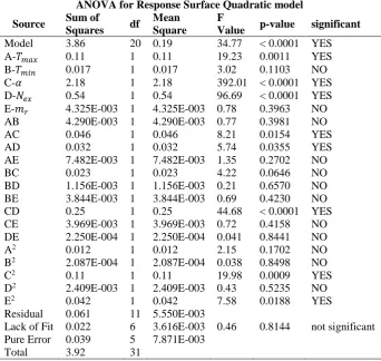
Table 5. Significance evaluation of the relationships between each SA parameters and the computational time.
ANOVA for Response Surface Quadratic model Source Sum of
Squares df
Mean Square
F
Value p-value significant
Model 3.86 20 0.19 34.77 < 0.0001 YES
A-𝑇𝑚𝑎𝑥 0.11 1 0.11 19.23 0.0011 YES
B-𝑇𝑚𝑖𝑛 0.017 1 0.017 3.02 0.1103 NO
C-𝛼 2.18 1 2.18 392.01 < 0.0001 YES
D-𝑁𝑒𝑥 0.54 1 0.54 96.69 < 0.0001 YES
E-𝑚𝑟 4.325E-003 1 4.325E-003 0.78 0.3963 NO
AB 4.290E-003 1 4.290E-003 0.77 0.3981 NO
AC 0.046 1 0.046 8.21 0.0154 YES
AD 0.032 1 0.032 5.74 0.0355 YES
AE 7.482E-003 1 7.482E-003 1.35 0.2702 NO
BC 0.023 1 0.023 4.22 0.0646 NO
BD 1.156E-003 1 1.156E-003 0.21 0.6570 NO
BE 3.844E-003 1 3.844E-003 0.69 0.4230 NO
CD 0.25 1 0.25 44.68 < 0.0001 YES
CE 3.969E-003 1 3.969E-003 0.72 0.4158 NO
DE 2.250E-004 1 2.250E-004 0.041 0.8441 NO
A2 0.012 1 0.012 2.15 0.1702 NO
B2 2.087E-004 1 2.087E-004 0.038 0.8498 NO
C2 0.11 1 0.11 19.98 0.0009 YES
D2 2.409E-003 1 2.409E-003 0.43 0.5235 NO
E2 0.042 1 0.042 7.58 0.0188 YES
Residual 0.061 11 5.550E-003
Lack of Fit 0.022 6 3.616E-003 0.46 0.8144 not significant Pure Error 0.039 5 7.871E-003
Total 3.92 31
Table 6. Optimal values of SA parameters obtained by DOE.
Fig 2. The history of the convergence of the proposed SA of the solution of the problem j30 (Num. 36) (vertical axis: the value of the objective function, horizontal axis: number of iterations).
SA parameters 𝑻𝒎𝒂𝒙 𝑻𝒎𝒊𝒏 𝜶 𝑵𝒆𝒙 𝒎𝒓
Optimal values 15 0.07 0.92 8 2
1500 2000 2500 3000 3500 4000 4500
0 50 100 150 200
Table 7. Results of solution of 36 problems with 30 activities by the proposed SA.
Pro. num. Size WCT BCT ACT WOF BOF AOF j M S w
1 30 1 2 2 0/433 0/306 0/386 2454 2451 2452
2 30 2 2 2 0/546 0/531 0/535 3117 3112 3114
3 30 3 2 2 0/779 0/425 0/578 4121 4107 4114
4 30 4 2 2 0/774 0/478 0/664 4333 4313 4326
5 30 1 3 2 0/355 0/267 0/308 2452 2451 2451
6 30 2 3 2 0/759 0/209 0/456 3110 3099 3103
7 30 3 3 2 0/469 0/367 0/364 4100 4098 4099
8 30 4 3 2 0/557 0/34 0/451 4311 4302 4307
9 30 1 4 2 0/498 0/369 0/424 2456 2451 2454
10 30 2 4 2 1/029 0/735 0/891 3085 3078 3082
11 30 3 4 2 1/238 0/455 0/787 4109 4090 4097
12 30 4 4 2 0/881 0/308 0/540 4274 4259 4266
13 30 1 2 3 0/892 0/852 0/878 1648 1647 1647
14 30 2 2 3 1/252 0/571 0/929 2051 2037 2044
15 30 3 2 3 0/93 0/884 0/779 2885 2851 2863
16 30 4 2 3 0/905 0/851 0/767 3041 3024 3031
17 30 1 3 3 0/986 0/954 0/922 1646 1644 1645
18 30 2 3 3 0/988 0/603 0/751 2046 2038 2042
19 30 3 3 3 1/462 0/928 1/144 2856 2844 2851
20 30 4 3 3 0/861 0/302 0/628 3030 3009 3019
21 30 1 4 3 1/154 0/99 0/957 1645 1644 1645
22 30 2 4 3 1/349 0/828 1/166 2034 2025 2029
23 30 3 4 3 1/632 1/347 1/219 2834 2828 2832
24 30 4 4 3 0/943 0/393 0/623 2998 2987 2993
25 30 1 2 4 1/294 1/045 1/161 1071 1066 1069
26 30 2 2 4 1/237 1/158 1/211 1401 1394 1397
27 30 3 2 4 2/674 1/359 1/816 1971 1961 1966
28 30 4 2 4 1/021 0/445 0/707 2211 2112 2154
29 30 1 3 4 1/313 0/998 1/199 1068 1065 1066
30 30 2 3 4 1/341 0/921 1/185 1399 1399 1399
31 30 3 3 4 1/275 1/09 1/113 1956 1951 1953
32 30 4 3 4 0/817 0/444 0/684 2117 2098 2108
33 30 1 4 4 1/703 1/165 1/449 1068 1065 1067
34 30 2 4 4 1/474 0/862 1/108 1387 1373 1380
35 30 3 4 4 1/531 1/143 1/388 1955 1941 1947
36 30 4 4 4 0/702 0/458 0/615 2095 2085 2090
Total - - - - 2/674 0/209 0/855 - - -
Table 8. Results of solution of j60 problems by the proposed SA.
Pro. num. Size WCT BCT ACT WOF BOF AOF J M S w
37 60 3 3 3 0/866 0/503 0/637 5751 5727 5735
38 60 4 3 3 0/704 0/482 0/498 5784 5753 5763
39 60 3 4 3 1/387 1/325 1/075 5737 5709 5720
40 60 4 4 3 0/866 0/27 0/637 5751 5727 5735
41 60 3 3 4 1/213 0/728 0/972 3953 3940 3945
42 60 4 3 4 0/276 0/115 0/172 4321 4291 4311
43 60 3 4 4 1/872 1/164 1/245 3953 3915 3936
44 60 4 4 4 0/267 0/069 0/191 4309 4261 4281
Total - - - - 1/872 0/069 0/678 - - -
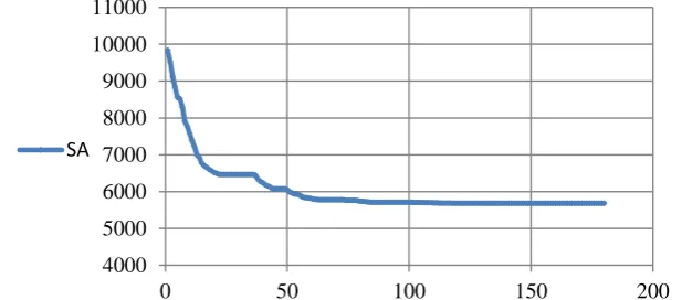
Fig 3. The history of the convergence of the proposed SA of the solution of the problem j60 (Num. 37) (vertical axis: the value of the objective function, horizontal axis: number of iterations).
As a result, our proposed SA was able to solve the problems with 30 and 60 activities in acceptable times. The convergence history shows the performance of the artificial intelligence of the algorithm in which the convergence rate is acceptable.
6. Conclusions
In this paper, the material allocation to the warehouse problem was modeled as a second problem besides the material procurement problem (MPS-MAW) which was not considered in the literature. In addition, the warehouse was considered as one place with the unlimited capacity in most of the papers, which is an unreal assumption in the real world. To overcome this issue, we developed MPS-MAW by considering multiple warehouses, which were unlimited at each period, however, these capacities were limited at the whole of the horizon planning with the objective function, which aims to consider the fair material distribution to the warehouses. By adding the new objective function besides the ordering and material transportation costs, not only the materials were allocated to the proper warehouses but also their assignments to the warehouses were leveled in order to maximize the utility of each warehouse. In order to solve this NP-hard problem, SA optimization algorithm was proposed in which the movement towards the neighborhood solution was improved by considering the mutation rate parameter, which was responsible to generate the solutions with high quality. Also, the encoding of the decision variables that was done by adding the auxiliary variable decreased the complexity of the modeling. Moreover, the solution of the small problem and comparing the results with the outputs of the exact method showed the validation of the proposed SA. Then, the outputs of DOE showed that the
4000 5000 6000 7000 8000 9000 10000 11000
0 50 100 150 200
impact of each SA parameters on the computational results. Finally, by the optimum values of the SA parameters, the large problems with the size of 30 and 60 activities, 1 to 4 materials, 2 to 4 suppliers and 2 to 4 warehouses were solved in acceptable times. For future studies, the MPS-MAW with considering the capacity of each warehouse at each period is suggested that is very real. Another suggestion can be using the other metaheuristics in order to compare each performance with our proposed model. The advanced modeling of the warehouses can be considering them as a 2-dimensional or multi-dimensional shape that each material must satisfy the geometry-related constraints.
References
[1] Caron, F., Marchet, G., & Perego, A. (1998). Project logistics: integrating the procurement and construction processes. International journal of project management, 16(5), 311-319.
[2] Chen, S. M., Chen, P. H., & Chang, L. M. (2012). Simulation and analytical techniques for construction resource planning and scheduling. Automation in construction, 21, 99-113.
[3] Dixit, V., Srivastava, R. K., & Chaudhuri, A. (2014). Procurement scheduling for complex projects with fuzzy activity durations and lead times. Computers & industrial engineering, 76, 401-414.
[4] Tabrizi, B. H., & Ghaderi, S. F. (2016). Simultaneous planning of the project scheduling and material procurement problem under the presence of multiple suppliers. Engineering optimization, 48(9), 1474-1490. [5] Tabrizi, B. H., & Ghaderi, S. F. (2016). A robust bi-objective model for concurrent planning of project
scheduling and material procurement. Computers & industrial engineering, 98, 11-29.
[6] Zoraghi, N., Najafi, A. A., & Akhavan Niaki, S. T. (2012). An integrated model of project scheduling and material ordering: a hybrid simulated annealing and genetic algorithm. Journal of optimization in industrial engineering, 5(10), 19-27.
[7] Zoraghi, N., Shahsavar, A., & Niaki, S. T. A. (2017). A hybrid project scheduling and material ordering problem: Modeling and solution algorithms. Applied soft computing, 58, 700-713.
[8] Tabrizi, B. H. (2018). Integrated planning of project scheduling and material procurement considering the environmental impacts. Computers & industrial engineering, 120, 103-115.
[9] Habibi, F., Barzinpour, F., & Sadjadi, S. J. (2019). A mathematical model for project scheduling and material ordering problem with sustainability considerations: A case study in Iran. Computers & industrial engineering, 128, 690-710.
[10]Kirkpatrick, S., Gelatt, C. D., & Vecchi, M. P. (1983). Optimization by simulated annealing. science, 220(4598), 671-680.
[11]Hwang, C. R. (1988). Simulated annealing: theory and applications. Acta applicandae mathematicae, 12(1), 108-111.
[12]Ingber, L. (1993). Simulated annealing: Practice versus theory. Mathematical and computer modelling, 18(11), 29-57.
[13]Szu, H., & Hartley, R. (1987). Fast simulated annealing. Physics letters A, 122(3-4), 157-162.
[14]Khosravi, P., Alinaghian, M., Sajadi, S. M., & Babaee, E. (2015). The periodic capacitated arc routing problem with mobile disposal sites specified for waste collection. Journal of applied research on industrial engineering, 2, 64-76.