Automatic Generation Control–An Enhanced Review

Automatic Generation Control–An Enhanced

Review

Rajesh Singh Shekhawat#1, Dr. Shelly Garg*2

#_{Research scholar, Department of Electrical Engineering, IIET, Kurusetra Unversity, Kurushetra, Haryana, INDIA} 2

Principal, IIET, Kurusetra Unversity, Kurushetra & University, Haryana, INDIA

Abstract— In this paper explanation about automatic generation control and its equivalent model with the help of MATLAB/Simulink. Power system operation active and reactive power demands are never steady and they continually vary with day to day. Generation must, therefore, be continuously changed with the active power demand. Reduce the machine speed will change consequently change in frequency. Power system frequency regulation entitled load frequency control (LFC), as a serious operate of automatic generation control (AGC), one of the necessary control issues in electric power system control and operation. The conventional frequency deviation on the far side bound limits will directly impact on grid operation and system dependability. A frequency deviation will injury equipment’s, degrade load performance as a result of the transmission lines to be overload and may interfere with system protection schemes associate degree ultimately result in an unstable condition for the power system. Maintaining frequency and power interchanges with neighbour area is primary objectives of an LFC. The main objectives are to control error signal and it is known as area control error (ACE), that represents the important power imbalance between generation and load, and could be a linear combination of power interchange and frequency deviations.

Keywords— Proportional Integral (PI), Area Control Error (ACE), Automatic Generation Control (AGC), Speed Governing System.

I. INTRODUCTION

ACE is employed to perform associate degree input control signal for a typically proportional integral (PI) controller. Looking on the control characteristics, the ensuing output control signal is conditioned by limiters, delays and gain constants. This control signal is then distributed among the LFC participant generator units in accordance with their participation factors to produce applicable control commands for set points of such that plants. The errors in frequency and net power interchange to be corrected by calibration the integral controller settings. Calibration of the dynamic controller is a vital issue to get optimum LFC performance. Correct calibration of parameters is required to get smart control action. [2]

The frequency control is changing into additional vital these days thanks to the increasing size, the ever-changing structure of complicated interconnected power systems. The controllers are set for a particular operating condition and they are responsible for small changes in the system without change in frequency and voltage exceeding the set limit.[6] Therefore, in the modern interconnected grid, LFC plays a basic role, as associate degree adjunct service, in supporting power exchanges and providing higher conditions for the electricity commerce.[

II. MODELOFSINGLEAREASYSTEM To know the load frequency control drawback, we have a tendency to think about one thermal system activity an isolated load.

For LFC scheme of single generating unit has basically three parts:

A. Turbine speed governing system B. Turbine

C. Generator and load.[3]

A. Model Speed Governing System

Fig. 1 represents schematically the speed governing system of a steam turbine.

The speed governing system consists of the following parts:

mechanism moves downwardly and the other way around.

2) Linkage Mechanism: ABC and CDE are the rigid links pivoted at B and D respectively. The mechanism provides a movement to the control valve within the proportion to the modification in speed. Link 4 provides a feedback from the steam valve movement.

3) Hydraulic Amplifier: This consists of the piston and pilot valve. Low power level pilot valve movement that is regenerate into high power level piston valve movement is critical to open or shut the steam valve against air mass steam.

4) Speed Changer: With the help of speed changer it maintains steady state power output setting for the turbine. Its downward movement opens the upper pilot valve so that more steam is admitted to the turbine under steady conditions. The reverse happens for upward movement of speed changer.

5) Model of Speed Governing System: Assume that the system is initially operating under steady conditions, the linkage mechanism is stationary and pilot valve is closed, steam valve opened by a definite magnitude, turbine running at constant speed with turbine power output balancing the generator load.

Let the operating conditions be characterized by f 0 = System frequency (speed)

PG0 = Generator Output = turbine output (neglecting

generator loss)

yG0 = Steam Valve Setting.

Now, a linear incremental model around these operating conditions is obtained.

Let the purpose A on the linkage mechanism be affected downward by a little quantity yA. It’s a

command that causes the turbine power output to alter and might thus, be written as

C C

A

K

P

y







(1)

Where-



P

_Cis the commanded increase in power. The command signal



P

_C sets into motion a sequence of events. The pilot valve moves upwards, high pressure oil flows on to the top of the main piston moving it downwards; the steam valve opening consequently increases, the turbine generator speed increases, i.e., the frequency goes up. Let us model these events mathematically

Two factors contribute to the movement of C:

(a)



y

_A Contributes

y

_A

or

K

y

_A

l

l

_

_

_













1 1

2

(i.e. upwards) of



K

₁

K

_C



P

_C where K1, Kc are

constants.

(b) Increased frequency



f

causes the fly balls to move outwards so that B moves downwards by a proportional amount

K

₂/



f

. The consequent movement of C with A remaining fixed at



y

_Ais

f

K

f

K

l

l

l

_

_

_











 

2 2

1 2 1

'

.

The net movement of C is therefore,

f

K

P

K

K

y

_C





_C



_C







_{1 2} (2)

where K2 is a constant.

The movement of D,



y

_D is the amount by which the pilot valve opens. It is contributed by



y

_C and

E

y



can be written as

E C

D

K

y

K

y

y











_{3 4} (3)

Where K3 and K4 are constants.

E

y



is the movement of point E.

The movement



y

D depending upon its sign

opens one of the parts of the pilot valve admitted high pressure oil into the cylinder thereby moving the main piston and opening the steam valve by

E

y



.

Certain Assumptions created are: -

i) Inertial reaction forces of main piston and steam valve area unit negligible compared to the forces exerted on the piston by high pressure oil. ii) Due to (i) higher than, the speed of oil admitted to the cylinder is proportional to part opening



y

_D

.

The volume of oil admitted to the cylinder is so proportional to the time integral of



y

_D

The movement



y

Eis obtained by dividing the

oil volume by the realm of the cross-sectional of the piston. Thus,















t

o

D

E

K

y

dt

y

5 (4)

positive movement



y

_D causes negative movement

E

y



accounting for the negative sign used in (3).

Taking the Laplace transform of equations, we get

)

(

)

(

)

(

s

K

₁

K

P

s

K

₂

F

s

y

_C





_C



_C







(5)

)

(

)

(

)

(

s

K

₃

y

s

K

₄

y

s

y

_D





_C





_E



(6)





s

s

y

K

s

y

D E

)

(

)

(



5







(7)

Eliminating yD(s) from (7), we get



(

)

(

)



)

(

5 _{3 4}

s

y

K

s

y

K

s

K

s

y

_E







_C





_E



(8)

Also eliminating yC(s) from (8), we get







(

)

(

)

(

)



)

(

5 _{3 1 2 4}

s

y

K

s

F

K

s

P

K

K

K

s

K

s

y

_E







_C



_C









_E



(9)

s

s

F

K

K

K

s

s

P

K

K

K

K

s

K

K

s

y

C C

E

)

(

)

(

1

)

(

5 4



3 1 5





3 2 5













 



(10) or





s

K

K

s

F

K

s

P

K

K

K

K

s

y

_E C C













4 5 2 1 5

3

(

)

(

)

)

(

(11) or

s

K

K

s

F

K

K

K

s

P

K

K

K

K

s

y

C C C E

























4 5 1 2 1 5 3

)

(

)

(

)

(

(12) or























C C C E

K

K

K

K

s

K

K

K

K

K

K

s

F

R

s

P

s

y

1 5 3 1 5 3 4 5

)

(

1

)

(

)

(

(13) or 4 1 3 5 4

1

)

(

1

)

(

)

(

_K

K

K

K

K

K

s

s

F

R

s

P

s

y

C C E











 











(14) or





























_

_

_





s

T

K

s

F

R

s

P

s

y

g g C E

1

)

(

1

)

(

)

(

(15) Where 2 1

K

K

K

R



C

= speed regulation of governor

4 3 1

K

K

K

K

K

C

g



= gain of speed governor

5 4

1

K

K

T

_g



= time constant of speed governor

Equation (15) can be represented in the form of block diagram as follows:

Figure 2 Block Diagram of Governor Model B. Turbine model

The model requires a relation between changes in power output of the steam turbine to changes in its steam value opening



y

_E(s).The response of a non-reheat turbine can be approximated by a single time constant Tt and is given by

)

(

1

1

)

(

y

s

s

T

s

P

_E

t

m



_





(16)

Where



y

_E

(

s

)

= steam valve opening

)

(

s

P

_m



= Laplace transform of



y

_m, the change in power developed by the turbine.

Tt = time constant of turbine (generally 0.25 sec or

so).

C. Model of Generator

Assuming generator to be loss free, the mechanical power input to the generator is equal to the electrical power output.

) ( )

D. Model of Generator with load

The increment is power input to the generator – load system is



P

_G





P

_D where



P

_G





P

_T. This increment in power input to the system is accounted for in two ways:-

(i) Rate of increase of stored kinetic energy in the generator rotor. At scheduled frequency

 

f

o , the stored energy is

)

(

sec

KJ

kw

P

H

W

_keo





_r



(17) Where Pr is the KW rating of the turbo – generator

and H is defined as its inertia constant.

The kinetic energy being proportional to square of speed, the kinetic energy at a frequency f0+∆f is given by: 2



















o o _o

ke Ke

f

f

f

W

W



















_{r o}

f

f

P

H

1

2

Rate of change of kinetic energy is therefore

)

(

2

)

(

f

dt

d

f

HP

W

dt

d

o r

Ke





(18)

(ii) As the frequency changes, the motor load changes being sensitive to speed, the rate of change of load with respect to frequency i.e.



P

_D

/



f

can be regarded as nearly, constant for small changes in frequency



f

and can be expressed as

f

B

sf

f

P

_D





















(19)

Where the constant B can be determined empirically, B is positive for a predominantly motor load. Writing the power balance equation, we have

f

B

f

dt

d

f

P

H

P

P

o r D

G















2

(

)

(20)

Dividing throughout by PT and rearranging we get

f

pu

B

f

dt

d

f

H

pu

P

pu

P

_G





_D



_o









(

)

(

)

2

(

)

(

)

(21)

Taking the Laplace transform, we can write



F

(

s

)

as

s

f

H

B

s

P

s

P

s

F

o D G

2

)

(

)

(

)

(













Or





_





























p p D G

T

s

K

s

P

s

P

s

F

1

)

(

)

(

)

(

(22) Where o p

f

B

H

T



2

= power system time constant

B

K

p

1



= power system gain

Equation (22) can be represented in block diagram form as shown in figure below

Fig. 3 Block diagram representation of generator load model

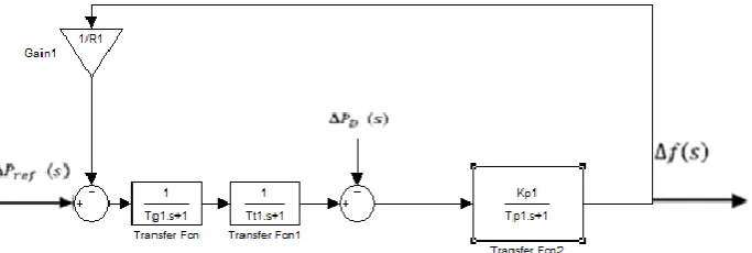
E. Complete Modelling of AGC in single area system

In this section, the analysis of load frequency control of one space grid is conferred. the entire system to be thought of for the look of controller is shown in Figure four. The system response has been obtained for uncontrolled and controlled system.

1) Steady state response

In uncontrolled case, speed changer has fixed settings, i.e. ∆Pref = 0

For step load change =∆PD

Laplace transform of it is ∆Pref = 0

Now from block diagram shown in Figure 3, system equation can be written as

∆𝑃

_𝑟𝑒𝑓

−

_𝑅1

∆𝑓 ∗ 𝐾

_𝐺

. 𝐾

_𝑇

− ∆𝑃

_𝐷

= ∆𝑓

(23) Laplace transform

∆𝑓(𝑠) =

𝐾𝑃

Figure 4 Complete block diagram of single area Thermal system Using the final value theorem

∆𝑓

𝑠𝑠

= lim

𝑠→0

𝑠∆𝑓 𝑠 =

𝑠.𝐾𝑃

1+_𝑅1𝐾𝑃.𝐾𝐺.𝐾𝑇 ∆𝑃𝐷

𝑠 (25)

=

𝐾𝑃∆𝑃𝐷

1+𝐾𝑃_𝑅

= −

∆𝑃𝐷

1+_𝑅1 (26) If β = [1 + 1/R] p.u. MWHz

Then

∆𝑓

_𝑠𝑠

= −

∆𝑃𝐷

𝛽 (27)

Where β is called area frequency response characteristic (AFRC). Thus, in uncontrolled case the steady state response has constant error.

2) Dynamic response

The dynamic response of a single area thermal system for a step load is calculated in this section. By taking inverse Laplace transform of equation (23), the frequency can be calculated in time domain ∆f (t). However, as KG, KT, Kp contain at least one

time constant each, the denominator will be of third

order, resulting in unwieldy algebra.

(Tg <<Tt<<Tp) where Tp is generally 20 s. Tg≈ Tt ≤ 1

s, thus assume Tg = Tt = 0 and the dynamic

frequency response can be calculated as

∆𝑓 𝑠 =

𝐾𝑃 1+𝑠𝑇𝑃 1+_𝑅1 𝐶

1+𝑠𝑇𝑃

∗

∆𝑃𝐷

𝑠 (28)

Above equation can also be written as

∆𝑓 𝑆 = −∆𝑃

_𝐷

∗

𝑅.𝐾𝑃 𝑅+𝐾𝑃

(

1 𝑠

−

1

𝑠+𝑅+𝐾𝑃_{𝑅.𝑇𝑃}

)

(29)

Taking inverse Laplace transform of above equation

∆𝑓 𝑡 = −∆𝑃

_𝐷

∗

𝑅.𝐾𝑃

𝑅+𝐾𝑃

[1 − 𝑒

−𝑡 𝑅+𝐾𝑃 𝑅.𝑇𝑃

]

(30)

Thus the error =

𝑒

−𝑡 𝑅+𝐾_𝑅.𝑇𝑃

𝑃 this persists in uncontrolled case.

Model of uncontrolled single area is shown in Figure .5.

Fig. 5 Block diagram model of single area Thermal System

III.MODELLING OF TWO AREA SYSTEM

A. Tie line model

The power flow over the line is

)

(

sin

_{1 2}

2 1 12









X

V

V

P

(31)

12

P = Power transfer from system 1 to system 2

1

V & V2 = voltage magnitudes at ends 1 and 2

1

 &₂= phase angles of voltages V1 and V2.

X = reactance of tie line

For small deviations in angles ₁ and₂, the change in power transfer P₁₂ is

) (

) (

cos 1 2 1 2

2 1

12     



X V V P

(32)

The synchronizing coefficient T of tie line is defined as

𝑇

₁₂

=

𝑉1 |𝑉2|

𝑋

cos(∆𝛿

1

− ∆𝛿

2

)

(33)

Then

∆𝑃

12

= 𝑇

12

(∆𝛿

1

− ∆𝛿

2

)

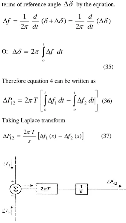
(34)

The frequency deviation



f

can be expressed in terms of reference angle





by the equation.

)

(

2

1

)

(

2

1

_





















dt

d

dt

d

f

Or









t

o

dt

f





2

(35) Therefore equation 4 can be written as



























t

o t

o

dt

f

dt

f

T

P

12

2



1 2 (36)

Taking Laplace transform



( ) ( )



2

2 1

12 f s f s

s T

P   

  (37)

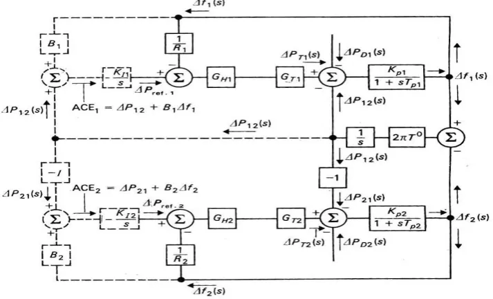
Figure 6 Linear representation of tie-line B. Implementation of Area Control Error in Model

The control signals (for each area) are proportional to the change in frequency as well as change in tie line power. As in the case of single

area systems, integral control is preferable because it gives zero steady state error [6]. The area control errors for a two area system are given by

1 1 12

1

P

B

f

ACE









₍₃₈₎

2 2 12

2

P

B

f

ACE









₍₃₉₎

where

ACE1 = Area control error of system 1

ACE2 = Area control error of system 2

P12 = Change in power transferred from 1 to 2

(+ve or –ve) P12 = -P21

B1 and B2 is constants which specify the frequency

bias and are determined from knowledge of the size of the system.

The commands to the speed changers are of the form



P B f



dt K

P_ref 



  

 1 1 12 1 1

(40)



P B f



dt K

Pref 



  

 2 2 21 2 2

(41) The constants K1 and K2 are integrator gains. The

minus sign in the above equation is essential because the generation in each area must increase if either its frequency error or tie line power increment is negative.

Most of the time a control area is interconnected with many other areas through several tie lines. Let there be a total of m tie lines. Then for the ith control area, the net interchange is the sum of power transfer over all the m tie lines. The area control error ACEi

of the ith area should be proportional to total exchange of power and can be expressed as

i m

j

i ij

i

P

B

f

CE

A











1

(42) The tie line power data of all the lines are sampled continuously at sampling intervals of about 1 second or so. These data are added in an energy control centre and compared with desired interchange (decided earlier by mutual agreements). The total line power transfer error is added to frequency bias power transfer error is added to frequency bias error

i

i

f

B



to give the area control error. The ACE command is communicated to the speed changers of all the generators in the area.

Figure 7 Linear Model of Two-Area System IV.AGCSYSTEMWITHPICONTROLLER

The complete block is diagram shown in figure 8 models the complete frequency controller system. However the above configuration does not result in steady-state nominal value of the frequency. There is always some steady state error in frequency present in the system. To minimize the steady-state deviation in frequency, therefore, the secondary controllers are used. The best controller suited for this purpose is integral controller [21].

The modified diagram of an isolated power system used with integral controller is shown below:

Figure 8 Implementation of Integral Controller in single area system

V. METHODOFTUNNINGPID CONTROLLER

From last six decades research has been carried out on tuning of P-I-D controllers. Several methods have also been implemented. Maximum model based, i.e. they design the mathematical model of the system which is available to the designer. In fact, if

the mathematical model of the system is available, most of them perform better than conventional Ziegler-Nichols method. But the good thing in ZN method is that it does not need a mathematical model, but controller parameters can easily be chosen by experiment process. We would be discussing the three experimental techniques those come under the commonly known Ziegler-Nichols method.

The error signal e (t) is fed to the controller and also the controller generates output u (t). Since the capability of the controller to deliver output power is restricted, associate mechanism is required in between the controller and also the method, which is able to actuate the control signal. It should be a valve actuator to open or shut a valve; or a damper actuator to regulate the air flow through a damper. The controller thought of here could be a P-I-D controller whose input and output relationship is given by the equation:

𝑢 𝑡 = 𝑘

𝑝

𝑘 𝑡 𝜏

𝑑 𝑑𝑒 (𝑡)_𝑑𝑡

+

_𝜏1

𝑖

𝑒(𝜏)𝑑𝜏

𝑡

0 Our

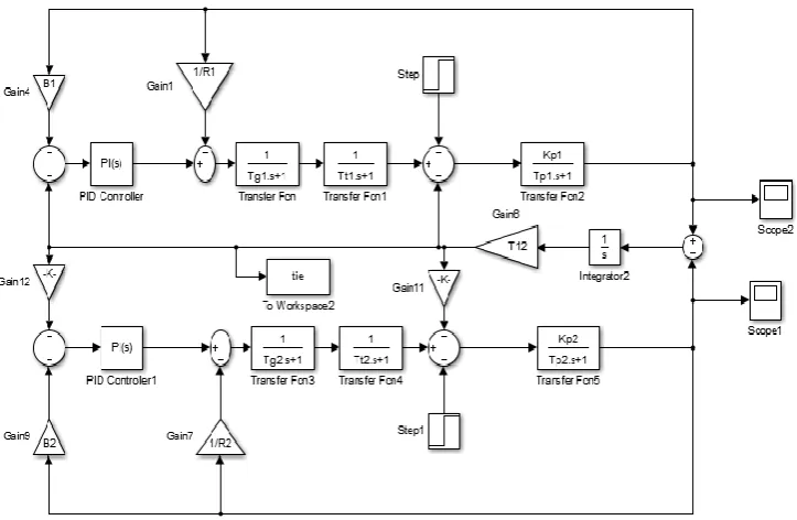
objective is to find out the optimum settings of the P,I,D parameters, namely kp, dτ and τi through

Figure 9 Simulink Model of Two Area Thermal System with PI Controller

 Reaction Curve Technique

 Closed Loop Technique (Continuous Cycling method)

 Closed Loop Technique (Damped oscillation method)

VI.SIMULATIONRESULT

The system which is investigated comprises a single area thermal system. The nominal system parameters of the system investigated are given in appendix.

The response for the frequency deviation of the single area system without controller is given in figure 10, and with conventional PI controller is given in figure 11. [15]

Figure 10 Simulated result of single area Thermal System without controller

Figure 11 Simulated result of single area System with PI controller

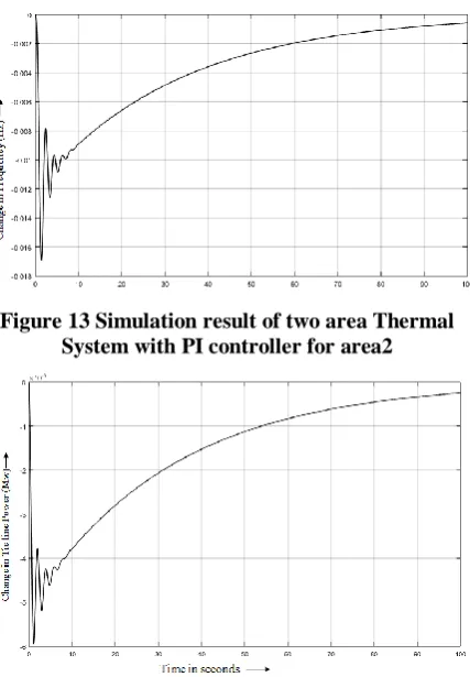
Figure 13 Simulation result of two area Thermal System with PI controller for area2

Figure 14 Simulation result of tie line power for two area Thermal System with PI controller Table 1 Time analysis parameters of simulations of single area Thermal system when 1% disturbance in this area

Parameters System Without Controller

System With PI controller

Undershoot(Hz) 0.031 0.031

Settling time(sec) Not settle 90

Table 2 Time analysis parameters of simulations of area 1 for Thermal-Thermal system when 1% disturbance in area1

Parameters System Without Controller

System With PI controller

Undershoot(Hz) 0.023 0.023

Settling time(sec) Not settle 100

Table 3 Time analysis parameters of simulations of area2 for Thermal-Thermal system when 1% disturbance in area1

Parameters System Without Controller

System With PI controller

Undershoot(Hz) 0.017 0.017

Settling time(sec) Not settle 110

Table 4 Time analysis parameters of simulations of tie line for Thermal-Thermal system when 1% disturbance in area1

Parameters System Without Controller

System With PI controller

Undershoot(Mw) 0.006 0.0059

Settling time(sec) Not settle 120

VII. CONCLUSION

In this Paper we studied the modelling of AGC in single area and two area of thermal power system. As steady state frequency deviation is not zero so PI controller is used to make it zero in this work. PI controller not gives fast steady state response also high amplitude oscillation present in output response. Tuning of PI controller is so complicated task so we need to design more controllers which will give fast response as well as less oscillation. So advance controller like Fuzzy logic controller approach can be applied for control the deviation in frequency.

VIII. ACKNOWLEDGMENT

This research paper was supported by B. K. Birla Institute of Engineering & Technology, Pilani. We thank to Dr. P. S. Bhatnagar from (Director, BKBIET, Pilani) who provided perceptions and expertise that assisted the research in a very precise manner.

I would also like to show our gratitude to the Dr. Shelly Garg (Principal, IIET) for sharing their pearls of intelligence with us during the course of this research. I am also immensely grateful to Dr. Shelly Garg my guide for their remarks on an earlier version of the manuscript. [1]

IX.REFERENCES

[1] Rajesh Singh Shekhawat "Infrared Thermography - A Review", International Journal of Engineering Trends and Technology (IJETT), V35(6),287-290 May 2016. ISSN:2231-5381. www.ijettjournal.org. published by seventh sense research group

[2] P.S.R. MURTHY, “Power System Operation and Control” McGraw Hill Publication, 1984.

[4] Lee, C. C. “ Fuzzy logic in control systems: Fuzzy logic control, part I” IEEE Transactions on Systems, Man, and Cybernetics, SMC 20, , pp. 404-418, 1990.

[5] P. Kundur “Power System Stability and Control” Mc-Graw-Hill publication, 1994.

[6] D. M. Vinod Kumar, “Intelligent controllers for Automatic Generation Control” IEEE, pp 557-574, 1998.

[7] Bjorn H. Bakken and Ove S. Grande, “Automatic Generation Control in a Deregulated Power System” IEEE Transactions on Power Systems, Vol. 13, No. 4, pp 1401-1406, November 1998.

[8] Alfred L. Guiffrida, Rakesh Nagi “Fuzzy set theory applications in production management research” a literature survey, Journal of Intelligent Manufacturing, Volume 9, Issue 1, pp 39-56, 1998.

[9] George Gross and Jeong Woo Lee “Analysis of Load Frequency Control Performance Assessment Criteria” IEEE transactions on power systems, vol. 16, no. 3, pp 520-525 August 2001.

[10] Katsuhiko Ogata “Modern Control Engineering” Fourth Edition 2002.

[11] J. Nanda, M. Parida and A. Kalam “Automatic generation control of a multi-area power system with conventional integral controllers” Melbourne, Australia TS13-Load and Frequency Control, vol. 2, In: Proc. AUPEC 2006. [12] Janardan Nanda, Ashish Mangla, and Sanjay Suri, “Some

New Findings on Automatic Generation Control of an Interconnected Hydrothermal System With Conventional Controllers” IEEE Transactions on energy conversion, vol. 21, no. 1, pp 187-194, March 2006.

[13] M.F. Hossaiin, T. Takahashi, M.G. Rabbani, M.R.I. Sheikh and M.S. Anower “Fuzzy-Proportional Integral Controller for an AGC in a Single Area Power System” 4th International Conference on Electrical and Computer Engineering ICECE 2006, pp 120-123, December 2006. [14] Ker-Wei Yu, Jia-Hao Hsu “Fuzzy Gain Scheduling PID

Control Design Based on Particle Swarm Optimization Method” Second International Conference on Innovative Computing, Information and Control, ICICIC.2007: 337-340, 2007

[15] Xinyi Ren, Fengshan Du, Huagui Huang, Hongyan Yan “Application of Fuzzy Immune PID Control Based on PSO

in Hydraulic AGC Press System” International Conference on Intelligent Human-Machine Systems and Cybernetics, Hangzhou, Zhejiang, pp: 427 - 430, 2009.

[16] S.K. Sinha, R.N.Patel, R.Prasad “Application of GA and PSO Tuned Fuzzy Controller for AGC of Three Area Thermal-Thermal-Hydro Power System” International Journal of Computer Theory and Engineering, 2(2): pp: 1793-8201, 2010.

[17] Guolian Hou, Lina Qin, Xinyan Zheng,Jianhua Zhang “Design of PSO-Based Fuzzy Gain Scheduling PI Controller for Four-Area Interconnected AGC System after Deregulation” Proceedings of the 2011 International Conference on Advanced Mechatronic Systems, Zhengzhou, China, August 11-13, 2011

[18] Hassan Bevrani, Senior Member, IEEE, and Pourya Ranjbar Daneshmand, “Fuzzy Logic-Based Load-Frequency Control Concerning High Penetration of Wind Turbines” IEEE SYSTEMS JOURNAL, VOL. 6, NO. 1, MARCH 2012 [19] Anju G Pillai, Meera Rose Cherian, Sarin Baby, Anish

Benny “Performance Analysis of Conventional and Intelligent Controllers In Power Systems With AGC,” International Journal Of Scientific & Engineering Research, Volume 4, Issue 8, August 2013

[20] Roohi Kansal1 Balwinder Singh Surjan, “Study of Load Frequency Control in an Interconnected System Using Conventional and Fuzzy Logic Controller,” international Journal of Science and Research (IJSR), Volume 3 Issue 5, May 2014

[21] Ramandeep Kaur, Jaspreet kaur, “PID Controller Based AGC under Two Area Deregulated Power System,” International Journal of Scientific & Engineering Research, Volume 6, Issue 6, June-2015

[22] D. K. Sambariya, Vivek Nath, “Optimal Control of Automatic Generation with Automatic Voltage Regulator Using Particle Swarm Optimization” Universal Journal of Control and Automation 3(4): pp 63-71, 2015