http://www.sciencepublishinggroup.com/j/wros doi: 10.11648/j.wros.20200901.12
ISSN: 2328-7969 (Print); ISSN: 2328-7993 (Online)
Evaluation of Spatial and Temporal Variability of Sediment
Yield on Bilate Watershed, Rift Valley Lake Basin, Ethiopia
Mesfin Amaru Ayele
1, *, Bogale Gebremariam
21Faculty of Hydraulic and Water Resources Engineering, Arba Minch University, Arba Minch, Ethiopia 2
Arba Minch Water Technology Institute, Arba Minch University, Arba Minch, Ethiopia
Email address:
*
Corresponding author
To cite this article:
Mesfin Amaru Ayele, Bogale Gebremariam. Evaluation of Spatial and Temporal Variability of Sediment Yield on Bilate Watershed, Rift Valley Lake Basin, Ethiopia. Journal of Water Resources and Ocean Science. Vol. 9, No. 1, 2019, pp. 5-14. doi: 10.11648/j.wros.20200901.12
Received: October 5, 2019; Accepted: December 24, 2019; Published: January 8, 2020
Abstract:
In the watershed, sediment yield spatially and temporarily variable due to the factors for instance land use land cover, type of soil, rainfall distribution, topography and management practices. The main objective of this study was to evaluate spatial and temporal variability of sediment yield on Bilate watershed using Soil and Water Assessment Tool (SWAT) model. Simulation carried out using meteorological and spatial data by dividing watershed in to 23 sub basins with 174 Hydrologic Response Units (HRUs). Model calibration period (2001-2010) and validation period (2011-2015) performed for monthly flow and sediment data using Sequential Uncertainty Fitting (SUFI-2) within SWAT Calibration of Uncertainty Program (SWAT-CUP). Model performance efficiency checked by coefficient of determination (R2), Nash-Sutcliffe model efficiency (ENS), and observationStandard Deviation Ratio (RSR) and percent bias (PBIAS) indicating good performance of model evaluation. From 23 sub basins, 11 were categorized from moderate to very high (10-26 ton/ha/year) sediment yielding sub basins and selected for sediment management scenarios. Scenarios result showed that average annual sediment yield reduction at entire watershed level after application of grassed waterway, filter strips, terracing and contouring were 54.45%, 30.13%, 63.26% and 59.56% respectively. Also, at treated sub basins level 68.04%, 38.41%, 80.58% and 77.42% of sediment reduction revealed after application of grassed waterway, filter strips, terracing and contouring respectively. It concluded that sediment yield reduction applying terracing was more effective than other conservation measures for affected sub basins.
Keywords:
SWAT Model, SUFI-2, Stream Flow, Sediment Yield, Management Scenarios, Bilate Watershed1. Introduction
Poor land use practices, inappropriate management systems and deforestation have play a major role causing soil erosion; land degradation, desertification and sedimentation problems in the watershed [1]. Sediment yield has strong correlation with soil type, land use/cover and slope of the watershed [2]. Effects of soil erosion in watershed especially on cultivated land are reduction of cultivable soil depth, loss of soil fertility and decrease of productivity, which finally may lead potentially widespread food shortages [3]. Watershed management, in its broader sense, considered an attempt to reduce nutrient damages, surface-run-off and sediment yield from watershed and to safeguard sustainable agricultural production [4]. Thus, inclusive understanding of hydrological
processes in watershed considered as a precondition for effective land and watershed management.
Sediment spatial variability analysis used for identification of sediment prone areas in the catchment and sediment yield reduction is possible by providing soil conservation measures [5]. Different researchers have classified sediment reduction methods into different categories for instance structural (check dams and terracing), vegetative and agronomic (filter strips, grassed waterways and reforestation) and management (contouring and rotational grazing) are frequently used sediment management practices [6, 7]. Spatial variaility of sediment yield evaluation carried out with semi-distributed models for instance SWAT and pixel-based model such as WATEM/SEDEM [8, 9].
watershed and River, it is necessary to evaluate and understand watershed sediment yield. Moreover, in the Bilate watershed there was no study conducted previousely regarding to spatial and teporal variability of sediment yield in sub basin scale.
Therefore, the purpose of this research study was to evaluate the spatial and temporal variability of sediment yield, develop sediment management scenarios for sediment prone areas and compare the scenarios result using Soil and Water Assessment Tool (SWAT model). SWAT model selected due to it is physically based semi distributed watershed model and ability to characterize complex watershed phenomena, simulate surface runoff, sediment yield and sediment management practices [10].
2. Materials and Methods
2.1. Study Area Description
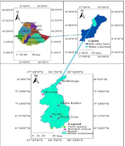
Bilate atershed is the sub-basin of the Rift Valley Lake Basin and located in the southwestern part of Ethiopia. It situated between 6°33’18’’ to 8°6’57’’ N latitudes and 37°47’14’’ to 38°20’14’’ E longitudes (Figure 1). Bilate River drains from northern part of the Lake Abaya drainage basin. The elevation of Bilate watershed ranges between 3359m a. m. s. l in the northern and 1156m a. m. s. l in the south and draiinage area of 5363 km2 at the entrance of Lake Abaya.
Figure 1. Location map of the Bilate watershed.
Average annual rainfall ranges from 1280-1339mm, 1061-1616mm and 769-956mm at upper, middle and lower part of the Bilate watershed respectively [11]. The maximum
exceeds 34.9°c in warm seasons and in the western highlands like Mount Ambarocho freeze in most times of the year [12]. The main land use/ cover of Bilate watershed are intensively and moderately cultivated land, grassland, shrub land, marshlands, forest, urban areas and exposed surface [11]. Dominant soil includes Vertic andosols, Chromic luvisols, orthic solonchaks, calcic xerosols, luvic phaeozems, pellic vertisols, dystric nitosols, eutric regosols and mollic nitosols, chromic vertisols, eutric nitosols, eutric fluvisols, calcic fluvisols, Leptosols and calcaric fluvisols [13].
2.2. Methodology
2.2.1. Data Collection and Analysis
Hydrological data (River discharge) of 17 years collected from Ministry of Water Irrigation and Energy. Meteorological data (precipitation, relative humidity, temperature, wind speed, sunshine hours) of 30 years collected from Ethiopia National Meteorological Agency. There are few days of measured sediment concentration data but long record of sediment data
generated by developing sediment-rating curve.
The spatial data for instance Digital Elevation Model (DEM), soil and land use land cover data were important in watershed modeling. A 30 m x 30 m resolution of Bilate watershed DEM downloaded from United States Geological Survey (USGS), SRTM (Shuttle Radar Topography Mission) web site http:/earthexplorer.usgs.gov/on 8 January 2019. Soil data collected from Ethiopian Ministry of water, irrigation and electricity (MoWIE) GIS department and the 2016 Rift valley land use/cover map with a 30m spatial resolution collected from Ministry of Agriculture (MoA). The collected data were analyzed by different statistical analysis were presented by means of graphs, figures and tables.
2.2.2. SWAT Model Inputs
SWAT model input data are soil map, land use/ cover map, DEM, slope and weather data for simulation whereas river discharge and sediment data are required for calibration and validation purposes in SWAT-CUP.
2.2.3. Watershed Delineation
SWAT allows the user to delineate watershed and sub basins using DEM to carry out advanced GIS functions to aid the user in dividing watersheds into several hydrological connected sub basins [10]. Delineation process includes five major steps: Digital Elevation Model (DEM) setup, stream definition, outlet and inlet definition, watershed outlet selection and definition and calculation of sub basin parameters. The DEM of Bilate watershed is loaded into Arc GIS 10.1 as grid format. Stream network was defined for the whole DEM and number of sub basins and stream network based on threshold area [14]. The smaller threshold area gives more detail of the drainage network, large numbers of sub basin and Hydrologic Response Unit (HRU). Threshold area of 13,500ha was taken for this work. The Bilate watershed outlet point manually added and selected for delineation. Finally, the Bilate watershed delineated with area of 5363km2 and23 sub-basins Figure 2 (a).
Once watershed delineated, then HRU analysis takes place. HRU analysis requires soil, land use/cover and slope data and divides sub basin in to number of HRU with a unique soil, land use/cover and slope combination. Produced HRU is crucial for simulation of SWAT model; because it determines how much the soil, land use and slope categorized will respond to precipitation, infiltration, surface runoff and sediment yield during the simulation. The soil land use and slope datasets were imported overlaid and linked with SWAT2012 databases. Delineated watershed and prepared land use were overlapped 100%. Land use map named into nine classes SWAT four-code letter Figure 2 (b). Also, delineated watershed and soil map overlapped 100% Figure 2 (c). Moreover, HRU analysis in SWAT model contains divisions of HRUs by slope classes. The slope discretization of watershed are 0-4, 4-8, 8-16 and >16% Figure 2 (d). To define the HRUs distribution there are two methods: one can be assigning only single HRUs for each sub basins considering the dominant soil, land use and slope. The second way is by assigning multiple HRUs for individual sub basins considering sensitivity of hydrologic process based on a certain threshold values of soli, land use and slope combinations. For this work, multiple HRUs selected. In multiple HRU definition 10 percent soil, 5 percent land use and 10 percent slope threshold used. Individual sub basin can have one or more HRUs defined within it. Finally, 174 HRUs for 23 sub basins created.
2.2.4. SWAT Model Simulation
The default input database files built and the required parameters values entered and edited manually then simulation taken to generate output of SWAT model. The simulated result cannot directly used for further analysis [15]. Therefore, the simulated result should evaluate through model sensitivity analysis, calibration and validation.
2.2.5. Model Parameters Sensitivity Analysis, Calibration and Validation
Modeler should be identifying sensitive parameters to allow the possible reduction in number of parameters that must be calibrated afterward reducing the computational time required for model calibration [16]. Flow and sediment sensitivity analysis performed by SWAT_CUP using SUFI-2 algorithm. Sensitivity analysis carried out for a period of twelve years, which includes two years warm-up period (January 1, 1999 - December 31, 2001) and ten years.
2.2.6. SWAT Model Performance Evaluation
SWAT model performance statistical measures includes Nash-Sutcliffe modeling efficiency (ENS), coefficient of determination (R2), percent bias (PBIAS) and Root mean square error observation standard deviation ratio (RSR) which were used to check the accuracy of river flow and sediment calibration and validation. cenario shows without consideration of management practices condition observed in watershed. It used as a reference point to know the effects of other scenarios sediment reduction results. Simulation of sediment yield in SWAT model with application of grassed waterway requires adjustment of grassed waterway parameters like length (GWAT_L), average slope (GWAT_S), depth (GWAT_D), manning’s roughness coefficient (GWAT_N), average width (GWAT_W) and linear factor for the channel sediment routing (GWAT_SPCON). Roughness coefficient of 0.35 (recommended value by Arnold et al., 2012) and average width of 30m was used. When slope length and steepness increase, there is a soil loss and surface runoff increase [13]. Terracing simulated in SWAT model by adjusting terracing parameters such as curve number (TERR_CN), slope length (TERR_SL) and USLE practice (TERR_P) factor.
Table 1. SWAT model performance evaluation criteria [17].
Rating R2 RSR E
NS
PBIAS
Flow Sediment
Very good 0.75 - 1 0 – 0.50 0.75 - 1 < 10% < 15%
Good 0.65 - 0.75 0.50 – 0.60 0.65 - 0.75 10% - 15% 15% - 30%
Satisfactory 0.50 - 0.65 0.6 – 0.70 0.50 - 0.65 15% - 25% 30% - 55%
Unsatisfactory < 0.60 ≤ 0.70 < 0.50 > 25% > 55%
For this study, appropriate curve number (TERR_CN), USLE practice (TERR_P) and 50% reduction of slope length was set based on land use/cover, soil and slope. Introducing filter strips on sediment prone sub basins can reduce sediment yield as width of strips reduced and increasing the width of strip beyond 30m [19]. In SWAT model filter strip parameters
width used to simulate this conservation practice for all HRUs of critical sub basins. Water breaks created after application of contour that reduces the formation of gullies and rills [20]. Simulation of SWAT model with application of contour carried out by adjusting USLE practice factor (CONT_P) and curve number (CONT_CN).
2.2.7. Sediment Yield Reduction Operations in SWAT Model In SWAT model, number of management operations, which used to reduce runoff and sediment yield in the affected sub basins. For this work, the sediment yield reduction methods like terracing, contouring, filter strip, grassed waterway selected and applied in SWAT model. Management practices applied in the critical sediment prone areas were more effective reduction of sediment yield than randomly assigning the conservation measures [18]. In this study each sub basins
sediment yield identified and grouped depend on their sediment rate (ton/ha/year). The sub basins having very high, high and moderate sediment yield selected for sediment reduction scenarios analysis.
For this study the developed scenarios includes grassed waterway, filter strips, terracing and contouring. Baseline calibration period (January 1, 2001 - December 31, 2010).
The sensitive parameters, which govern the watershed was btained and ranked according to their sensitivity rank. Calibration done by changing the model sensitive parameter values until simulated results much with observed data. Model validation carried out with independent set of measured flow and sediment data (January 1, 2011- December 31, 2015) without any further change of parameters.
Table 2. Summary of calibrated flow parameters.
Parameters Description Range value Calibration range Fitted values Rank
CN2 SCS runoff curve number 35-98 ±25% 0.026 1
CANMX Maximum canopy storage 0 - 10 0 - 10 1.125 2
GWQMN Threshold depth of water in the shallow aquifer for return flow to
occur 0 - 500 0 - 500 492.261 3
ALPHA_BF Alpha base flow recession constant 0 - 1 0 - 1 0.388 4
CH_K2 Effective hydraulic conductive of main channel 0 - 150 0 - 150 98.502 5
ESCO Soil evaporation compensation factor 0 - 1 0 - 1 0.110 6
RCHRG_DP Deep aquifer percolation fraction 0 - 1 0 - 1 0.164 7
PPERCO Phosphorus percolation coefficient 10 - 18 10 - 18 12.568 8
SMFMX Maximum melt rate for snow 0 - 10 0 - 10 7.532 9
3. Results and Discussions
3.1. Stream Flow Sensitivity Analysis
Depending on p-value and t-stat results obtained from sensitivity analysis using SUFI-2, the ranks of parameters assigned. P-value indicates significance of sensitivity and t- stat provides the measure of parameter sensitivity [21]. Larger t-stat in the absolute value means parameter is more sensitive and p-value closer to zero means parameter has more significance. Twenty parameters used to check sensitivity analysis and the nine more influential flow parameters from high to medium sensitive identified for further iterations in calibration process.
3.2. Stream Flow Calibration and Validation
The objective of calibration process is to create agreement
among the simulated and observed value by changing sensitive flow parameters in the recommended range.
Validation involves model run with unchanged flow parameters, which adjusted during calibration process. The flow calibration period (2001-2010) and validation period (2011-2015) result showed that a very good performance with R2 of 0.83, ENS of 0.78, RSR of 0.44 and PBIAS of-13.3% for
calibration and also R2 of 0.81, ENS of 0.74, RSR of 0.50 and
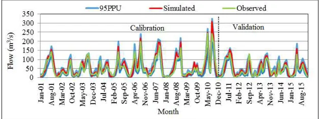
PBIAS of -14.6% for validation. Uncertainty measure of SUFI-2 indicated that P-factor of 0.74 and R-factor of 0.48 for calibration and P-factor of 0.72 and R-factor of 0.46 for validation. It means that about 74% of data of calibration and 72% of data of validation was bracketed by 95PPU band with a better strength of estimation (R-factor <1) for both cases. This indicates SWAT model has acceptable level of uncertainty for estimation of flow of Bilate watershed. Using monthly observed and simulated result, hydrograph developed for calibration and validation (Figure 3).
Figure 3 showed that peak simulated and observed flow occurs since August, 2010 and May, 2010 respectively. In addition, the hydrographs indicated that model slightly overestimated flow from watershed in most of the year and underestimated in some years.
Figure 4. Scatter plot of monthly observed and simulated flow.
From the scatter plot (Figure 4) it observed that more values distributed above 450 (1:1) line and shows model slightly overestimated the simulated flows.
3.3. Sediment Yield Sensitivity Analysis
Like flow, sediment sensitivity analysis applied to identify sensitive parameters that influence the modeling of sediment yield. Sediment sensitivity analysis carried out for 2 years warm-up period 1999 to 2001 and 10 years calibration period 2001 to 2010. Through sensitivity analysis of sediment yield seventeen sediment parameters were tested using SUFI-2 in SWAT-CUP.
Sediment yield validation conducted with independent sediment measured data for periods 2011 to 2015 without further change of calibration fitted parameters. Based on model performance evaluation criteria (Table 1), the sediment simulation result indicated that very good model.
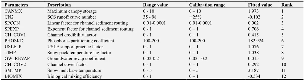
Based on the results obtained from sensitivity analysis, ranks of sediment parameters assigned depending on p-value and t-stat. Out of seventeen parameters, twelve were from high to medium sensitive parameters identified for sediment calibration process.
Table 3. Selected twelve sediment calibration parameters.
Parameters Description Range value Calibration range Fitted value Rank
CANMX Maximum canopy storage 0 - 10 0 – 10 1.973 1
CN2 SCS runoff curve number 35 - 98 ±25% -0.102 2
SPCON Linear factor for channel sediment routing 0.01-0.0001 0.01-0.0001 0.002 3
SPEXP Exponent factor for channel sediment routing 0 - 1 0 – 1 0.706 4
CH_COV1 Channel erodibility factor 0 - 1 0 – 1 0.415 5
PHOSKD Phosphorus partitioning coefficient 100-200 100-200 182.924 6
USLE_P USLE support practice factor 0 - 1 0 – 1 1.076 7
TIMP Snow pack temperature lag factor 0 - 1 0 – 1 1.038 8
GW_REVAP Groundwater revap coefficient 0.02-0.2 0.02 - 0.2 0.015 9
CH_COV2 Channel cover factor 0 - 1 0 – 1 0.292 10
SMTMP Snow melt base temperature 0 - 5 0 – 5 3.187 11
BIOMIX Biological mixing efficiency 0 - 1 0 – 1 -0.534 12
3.4. Sediment Yield Calibration and Validation
Sediment yield calibration carried out from 2001 to 2010 of sediment data. Sediment yield calibration and parameters adjustment continued iteratively until observed and simulated sediment yield fitted. efficiency level with R2 of 0.84, ENS of
0.78, PBIAS of 7.9% and RSR of 0.41 for calibration; R2 of 0.81, ENS of 0.73, PBIAS of -9.4% and RSR of 0.50 for
validation. Uncertainty measures of SUFI-2 indicated that p-factor of 0.72 and R-factor of 0.41 for calibration and P-factor of 0.80 and R-factor of 0.45 for validation, which shows acceptable level of uncertainty range.
From Figure 5 it was observed that peak simulated and observed sediment yield occurs since August, 2010 and May, 2010 respectively. The sediment graph (Figure 5) also indicated that model slightly overestimated sediment yield in most of the year and underestimated in some years. This is the same discussion with the flow hydrograph discussed in Figure 3because of the sediment yield is direct proportional to generated erosion and flow in the river.
3.5. Spatial and Temporal Variability of Sediment Yield in Watershed
Spatial and temporal variability of sediment yield in watershed because of the factors for instance land use/cover,
type of soil, rainfall distribution, and topography and management practices. Thus, in each sub basin the sediment yield was not uniform.
3.5.1. Spatial Variability
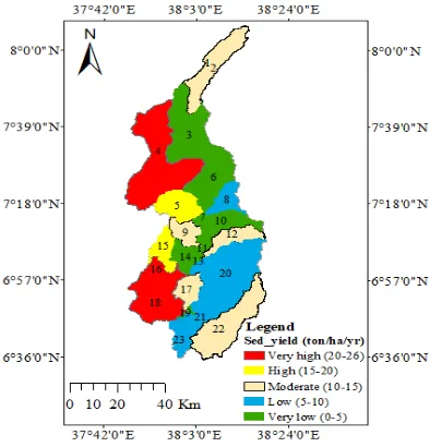
To get mean annual sediment yield spatially with sub basins level, SWAT model simulated annually for seventeen years sediment data. Spatial variability of sediment yield for Bilate watershed identified from the simulated sediment yield (Figure 6). The result showed the range was between 1.07 to 25.59 tons/ha/year with average sediment yield of 9.99 ton/ha/year (Table 4).
Table 4. Mean annual sediment yield of each sub basin.
Sub basin Sediment Yield (ton/ha/yr.) Sub basin Sediment Yield (ton/ha/yr.) Sub basin Sediment Yield (ton/ha/yr.)
1 12.20 9 13.42 17 12.98
2 11.72 10 4.74 18 23.85
3 1.17 11 1.69 19 1.08
4 25.95 12 10.14 20 6.76
5 18.21 13 3.18 21 8.49
6 3.38 14 1.07 22 14.77
7 1.71 15 16.51 23 6.61
8 9.24 16 20.98
Spatial variability of sediment yield map (Figure 6) was generated using mean annual sediment yield (Table 4) based on sediment yield potential
From the total twenty three sub basins (Figure 6), eleven sub basins producing sediment yield from very high to moderate (10-26 ton/ha/year) and identified as sediment prone areas. Out of eleven critical sub basins, three were very high (20-26 ton/ha/year), two were high (15-20 ton/ha/year) and six were moderately (10-15 ton/ha/year) sediment yielding sub basins.
Mean sediment yield of eleven identified sediment prone sub basins was 16.43 ton/ha/year and covers 55.6% of total
watershed area.
Figure 6. Spatial variability of sediment yield map for the Bilate watershed.
3.5.2. Temporal Variability
Temporal variability of sediment yield highly correlated with precipitation and surface runoff (Figure 7).
Figure 7. Temporal variability of sediment yield relation to precipitation and surface runoff.
From Figure 7 it was observed that high sediment observed during the months of April, May, June, July, August and September where as low sediment yield observed during October, November, December, January, February and March. The average temporal variable sediment yield was 4.89ton/ha.
3.6. Sediment Yield Reduction Methods
Once the sediment prone areas identified, then developing sediment reduction methods for affected sub basins was take place. In this study, four management operations (scenarios) were developed and compared with baseline scenario.
3.6.1. Baseline Scenario
3.6.2. Scenario I: Grassed Waterway
Introducing grassed waterways for the critical sediment prone sub basins with width of 30m, reduced average annual sediment yield from 16.43ton/ha/year to 5.25ton/ha/year
(68.04%) and at entire watershed level 9.99ton/ha/year to 4.55ton/ha/year (54.45%) reduced. In this scenario, all sediment prone sub basins changed from the category of very high, high and moderate to the low and very low sediment yielding.
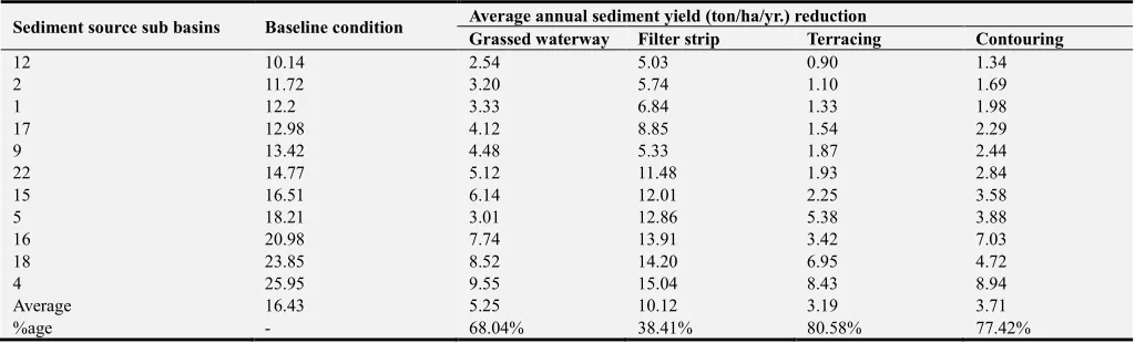
Table 5. Summary of developed scenarios result for eleven affected sub basins.
Sediment source sub basins Baseline condition Average annual sediment yield (ton/ha/yr.) reduction
Grassed waterway Filter strip Terracing Contouring
12 10.14 2.54 5.03 0.90 1.34
2 11.72 3.20 5.74 1.10 1.69
1 12.2 3.33 6.84 1.33 1.98
17 12.98 4.12 8.85 1.54 2.29
9 13.42 4.48 5.33 1.87 2.44
22 14.77 5.12 11.48 1.93 2.84
15 16.51 6.14 12.01 2.25 3.58
5 18.21 3.01 12.86 5.38 3.88
16 20.98 7.74 13.91 3.42 7.03
18 23.85 8.52 14.20 6.95 4.72
4 25.95 9.55 15.04 8.43 8.94
Average 16.43 5.25 10.12 3.19 3.71
%age - 68.04% 38.41% 80.58% 77.42%
3.6.3. Scenario II: Filter Strip
Applying filter strips with 10m width for the eleven sediment prone sub basins brought a slight reduction by38.41% (16.43ton/ha/year to 10.12ton/ha/year). At entire watershed level the reduction from 9.99ton/ha/year to 6.98ton/ha/year (30.13%). After application of filter strips, sediment prone sub basins changed from category of very high to high, high to moderate and moderate to a category of low.
3.6.4. Scenario III: Terracing
Simulation of terracing for the sediment prone sub basins significantly reduced sediment yield rate by 80.58% (16.43ton/ha/year to 3.19ton/ha/year) at treated sub basin level. In addition, at the entire watershed level, sediment yield reduced from 9.99ton/year to 3.67ton/year (63.26%). After
application of terraces all sediment prone sub basins changed to low and very low sediment yielding.
3.6.5. Scenario IV: Contouring
Simulation of contouring for sediment prone sub basins reduced sediment yield by 77.42% (16.43ton/ha/year to 3.71ton/ha/year) at treated sub basins level. At entire watershed level, sediment yield reduced by59.56% (9.99ton/year to 4.04ton/ha/year). After application of contours all sediment prone sub basins changed to low and very low sediment contributing sub basins.
3.7. Comparison of Scenarios Result
After all scenarios result analyzed, it is expected to compare and select best sediment reduction practice for affected sub basins.
Figure 8. Scenarios sediment yield reduction at treated sub basins level.
As shown in Figure 8, the sediment yield reduction after application of grassed waterway, filter strip, terracing and contouring were relatively consistent in all sub basins except
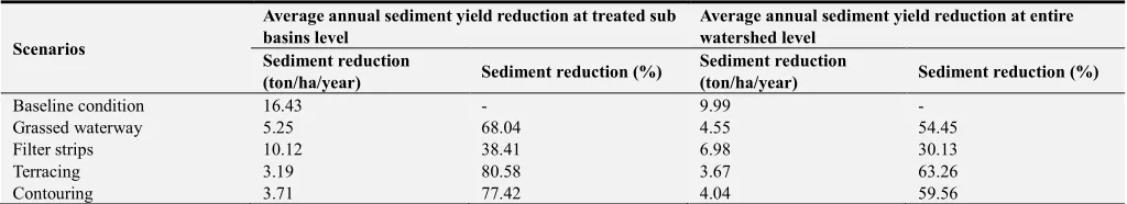
Table 6. Summary of scenarios result at treated sub basins level and entire watershed level.
Scenarios
Average annual sediment yield reduction at treated sub basins level
Average annual sediment yield reduction at entire watershed level
Sediment reduction
(ton/ha/year) Sediment reduction (%)
Sediment reduction
(ton/ha/year) Sediment reduction (%)
Baseline condition 16.43 - 9.99 -
Grassed waterway 5.25 68.04 4.55 54.45
Filter strips 10.12 38.41 6.98 30.13
Terracing 3.19 80.58 3.67 63.26
Contouring 3.71 77.42 4.04 59.56
As shown in Table 6, after simulation of terracing sediment yield reduction at entire watershed level 63.26% (9.99 to3.67ton/ha/year) and at treated sub basins level 80.58% (16.43 to 3.19ton/ha/year) observed. Sediment reduction at sub basin 18 and 5 than the other scenarios respectively. Terracing has best sediment reduction in all sub basins except sub basins 5 and 18. Filter strip has least sediment reduction in all sub basins.
Thus, terracing was relatively more sediment reduction practices on the majority of the affected sub basins than the other scenarios.
4. Conclusions
Rainfall runoff influenced soil erosion can expressively cause significant environmental degradation, reduce the soil fertility and productivity of cultivate land in watershed. In this study, spatial and temporal variability of sediment yield evaluation, identification of sediment prone areas, sediment reduction scenarios and their result comparison carried out using SWAT model. Based on watershed delineation, catchment area was 5363km2. Overlaying land use, soil and slope map performed to generate HRUs. Climate data from January 1987 - December 2015 were inputs for SWAT model simulation. The calibration and validation carried out from January 2001 - December 2010 and January 2011 - December 2015 respectively on monthly basis of flow and sediment data using automatic calibration with Sequential Uncertainty Fitting (SUFI-2) in SWAT- CUP. SCS curve number (CN2), threshold depth of water in the shallow aquifer for return flow to occur (GWQMN), maximum canopy storage (CANMX) and alpha base flow (ALPHA_BF) were catchment controlling flow parameters. During sediment calibration maximum canopy storage (CANMX), SCS curve number (CN2) and linear factor for channel sediment yield routing (SPCON) were more catchment controlling sensitive sediment parameters played major role in the calibration process for sediment yield.
Model performance efficiency checked by Nash-Sutcliffe model efficiency (ENS), coefficient of determination (R
2
), percent bias (PBIAS) and observation standard deviation ratio (RSR). Accordingly, the values of R2, ENS, RSR and PBIAS
vary between 0.79 - 0.85, 0.72 - 0.78, 0.41 - 0.61 and -14.6 - +11.6 respectively through calibration and validation for both discharge and sediment yield. These stated results indicated that model was soundly simulated the discharge and sediment yield. Spatial variability of sediment yield distribution ranges
from 1.07 to 25.59 ton/ha/yr. About 55.6% of total watershed area contributes average annual sediment yield rate of 16.43ton/ha/year and identified as sediment source areas. Temporal variability of monthly average sediment yield was 4.65ton/ha. The developed scenarios result showed that sediment yield reduction at entire watershed level after application of filter strips, grassed waterway, terracing and contouring were 30.13%,54.45% 63.26% and 59.56% respectively. Also at treated sub basins level 38.41%, 68.04%, 80.58% and 77.42% of sediment yield reduction observed after application of filter strips, grassed waterway, terracing and contouring respectively. Thus, the result indicating that terracing was relatively more sediment reduction practice than other conservation measures on the majority of the affected sub basins in Bilate watershed.
Statement on Conflicts of Interest
There is no conflict of interest.
References
[1] Allan, D., Erickson, D., and Fay, J. (1997). The influence of catchment land use on stream integrity across multiple spatial scales. Freshwater Biology, 37 (1), 149–161.
[2] Garcia-RuizJ, R. D.-R.-M. (2008). Flood generation and sediment transport in experimental catchments affected by land use changes in the central Pyrenees. pp. Hydrology, 245-260.
[3] Abegaz, G. (1995). Soil erosion assessment: Approaches, magnitude of the problem and issues on policy and strategy development (Region 3). Paper presented at the Workshop on Regional Natural Resources Management Potentials and Constraints, Bahir Dar, Ethiopia.
[4] Tripathi, M. P., Panda, R. K., & Raghuwanshi, N. S. (2004). Development of effective management plan for critical subwatersheds using SWAT model. Department of Soil and Water Engineering, Faculty of Agricultural Engineering, Indira Gandhi Agricultural Uni.
[5] Basson, G. R., & Rooseboom, A. (1999). Dealing with reservoir sedimentation: guidelines and case studies. International Commission on Large Dam Bulletin 115.
[7] Douglas G. Emerson, Aldo V. Vecchia, and Ann L. Dah. (2005). Evaluation of DrainageArea Ratio Method Used to Estimate Stream flow for the Red River of the North Basin, North Dakota and Minnesota. Scientific Investigations Report 2005–5017. U.S. Department.
[8] Chen, E. & Mackay, D. S. (2004). Effects of distribution-based parameter aggregation on a spatially distributed nonpoint source pollution model. J. Hydro. 295, 211–224.
[9] Verstraeten, G., Prosser, I. P. & Fogarty, P. (2007). Predicting the spatial patterns of hillslope sediment delivery to river channels in the Murrumbidgee catchment, Australia. J. Hydro. 334, 440–454.
[10] Arnold, J. G., Haney, E. B., Kiniry, J. R., Neitsch, S. L., Srinivasan, R., Neitsch, S. L., & Williams, J. R.. (2012). Soil and Water Assessment Tool (SWAT) theoretical documentation version 2012. Texas Water Resources Institute Technical Report No. 439, pp65.
[11] Demisse, M. (2015). Assessment of Climate Change Impact on Flood Frequency of Bilate River Basin.
[12] Sendabo, D. (2007). Analysis of biomass degradation as an indicator of environmental challenge of Bilate watershed using GIS techniques.
[13] Ayenew, T. (1998). The hydrogeological system of the Lake District basin, Central Main Ethiopian Rift valley, Free University of Amsterdam, the Netherlands, 259pp.
[14] Winchell, M., R., Srinivasan, R. Di Luzio, M. and Arnold, J. G. (2007). Arc SWAT Interface for SWAT2005. Grassland, Soil & Water Research Laboratory, USDA Agricultural Grassland, Soil & Water Research Laboratory, USDA Agricultural.
[15] White, K. L. & Chaubey. (2005). Sensitivity analysis, calibration, and validations for a multisite multivariable SWAT model. Journal of American Water Resources Association. 41: 1077–1089.
[16] Dilnesaw, A. (2006). Modeling of Hydrology and Soil Erosion of Upper Awash River Basin. Unpublished Ph. D. Thesis, University of Bonn.
[17] Moriasi D. N., Arnold J. G, Liew M. W., Bingner R. L., Haremel R. D. and Veith T. L. (2007). Model Evaluation Guidelines for Systematic Quantification of Accuracy in Watershed Simulations, Journal of American Society of Agricultural and Biological Engineers, 50: 885-900.
[18] Sharpley, A. N., Weld, J. L., Beegle, D. B., Kleinman, P. J., Gburek, W. J., Moore, P. A., & Mullins, G. (2003). Development of phosphorus indices for nutrient management planning strategies in the United States. Journal of Soil and Water Conservation, 58: 137-152.
[19] Arabi, M, Frankenberger, J. R., Enge, B. A. (2008). Representation of agricultural conservation practices with SWAT. Journal of Hydrological Processes, 22: 30423055.
[20] Manawko, W. (2017). Assessing Effectiveness of Watershed Management Options for Sediment Yield Reduction Using SWAT Model: A Case Study of the Proposed Middle Awash Dam Watershed, Ethiopia.

![Table 1. SWAT model performance evaluation criteria [17].](https://thumb-us.123doks.com/thumbv2/123dok_us/8484143.1714764/4.595.42.548.611.675/table-swat-model-performance-evaluation-criteria.webp)