Biological data and model development for management of longfinned eels

(1)

Project Report QO04015

Biological data and model

development for management of

longfinned eels

Simon D. Hoyle, Michael J. Hutchison,

Michelle J. Sellin, David Peel, David Mayer and Wayne D. Sumpton

(2)

QO04015 ISSN 0727 6281 ISBN 0 7345 1298 2 Agdex 476/10

Information contained in this publication is provided as general advice only. For application to specific circumstances, professional advice should be sought.

The Department of Primary Industries and Fisheries, Queensland, has taken all reasonable steps to ensure that the information contained in this publication is accurate at the time of production. Readers should ensure that they make appropriate inquiries to determine whether new information is available on the particular subject matter.

Copyright protects this publication. Except for purposes permitted by the Copyright Act, reproduction by whatever means is prohibited without prior written permission of the Department of Primary Industries and Fisheries, Queensland, and the Fisheries Research and Development Corporation. Inquiries should be addressed to:

Southern Fisheries Centre

Department of Primary Industries and Fisheries PO Box 76

(3)

Figures

Chapter Caption Page

Chapter 1 Figure 1: South-east Queensland eel survey age structure and index of abundance sampling sites.

3

Chapter 2 Figure 1: Mark recapture and ageing validation sites. 19 Chapter 4 Figure 1: An otolith from a twice OTC marked and then

recaptured wild eel viewed under reflected light (A) and UV light (B) with two OTC marks visible in the UV image.

48

Figure 2: An otolith from a tank held OTC marked eel viewed under reflected light (A) and UV light (B) with a single band of OTC visible in the UV image.

48

Figure 3: An otolith from Anguilla reinhardtii viewed under reflected light, showing annuli (A) the marine nucleus (N), freshwater check (F) and the edge of the otolith (E).

48

Figure 4: Plot of the relationship between somatic growth of wild longfinned eels and growth of otoliths to the OTC mark.

54

Figure 5: Plot of the relationship between somatic growth of wild longfinned eels and growth of otoliths measured to the edge (black diamonds), compared with plot of the relationship between somatic growth of wild longfinned eels and growth of otoliths to the OTC mark (white squares).

54

Figure 6: Plot of the relationship between somatic growth of longfinned eels and growth of otoliths to the OTC mark..

55

Figure 7: Plot of the relationship between somatic growth of longfinned eels and growth of otoliths to the OTC mark using pooled data for wild marked-recaptured eels and eels OTC tagged after being held in tanks for less than two months.

55

Figure 8: Plot of the relationship between somatic growth of eels held in tanks for 18 months and growth of otoliths measured to the ventral edge.

56

Chapter 5 Figure 1: Annual probability of differentiation versus length (mm) for Queensland and New South Wales, and annual probability of maturation versus length for Queensland.

69

Figure 2: Posterior estimates for female maturity parameters calculated from Burnett Creek eels: (a) maturity γ, (b) λ, (c) η.

69

Figure 3: Posterior estimates for male maturity parameters

calculated from Burnett Creek eels: (a) maturity γ, (b) λ, (c) η. 70 Figure 4:The posterior distributions of selected parameters for

Queensland: (a) a1, (b) a2, (c) b1, (d) diff gamma, (e) diff lamda, (f) diff nu, (g) total mortality, (h) sex ratio, (i) mean selectivity, (j) selectivity slope.

71

Figure 5: Posterior distributions for New South Wales growth and sexual differentiation: a) a2, b) b1, c) diff gamma, d) diff lambda, e) diff nu, f) total mortality, g) mean

selectivity, h) selectivity slope.

(5)

Figure 6: The posterior distributions of maturity parameters for New South Wales: (a and b) female and male maturity, (c and d) female and male maturity,(e and f) female and male maturity η.

73

Chapter 6 Figure 1: Queensland female long-finned eels at equilibrium: Relative egg production per recruit and yield per recruit at a range of exploitation rates and minimum legal sizes. a) Relative egg production per recruit. b) Relative yield-per-recruit declines at higher exploitation rates, depending on legal size. Minimum legal size affects yield-per-recruit more at high fishing pressures. c) Relative yield-per-recruit is greatest at high legal sizes and fishing pressures.

89

Figure 2: NSW female longfin eels at equilibrium: Relative egg production per recruit and yield per recruit at a range of exploitation rates and minimum legal sizes. a) Relative egg production per recruit. b) Relative yield-per-recruit as a function of legal size and fishing pressure. c) Relative yield-per-recruit at a range of minimum legal sizes and exploitation rates.

90

Figure 3: Queensland male longfin eels at equilibrium:

Relative spawning biomass per recruit and yield per recruit at a range of exploitation rates and minimum legal sizes. a) Relative spawning biomass per recruit. b) Relative yield-per-recruit increases with exploitation rate for all minimum legal sizes. c) Relative yield-per-recruit is greatest at high fishing pressure.

91

Figure 4: NSW male longfin eels at equilibrium: Relative spawning biomass per recruit and yield per recruit at a range of exploitation rates and minimum legal sizes. a) Relative

spawning biomass per recruit. b) Relative yield-per-recruit increases with exploitation rate for all minimum legal sizes. c) Relative yield-per-recruit is greatest at high fishing pressure.

92

Chapter 7 Figure 1: Screen capture of User worksheet. 102

Figure 2: Screen capture of Data worksheet. 106

Figure 3: Screen capture of Working worksheet. 107 Figure 4: Schematic diagram of model processes. Each cycle

through the model takes one year.

108

(6)

Tables

Chapter Caption Page

Chapter 1 Table A1: Adjusted average capture rates of large eels in dams, by site and type of aquatic macrophyte.

5

Table A2. Goodness of fit of the Poisson GLMs for eel captures.

6

Table A3. Adjusted average capture rates (per shot), by depth.

6

Table A4. Adjusted average capture rates (per shot), by stream physical habitat type.

6

Table A5. Adjusted average capture rates (per shot), by rocks.

7

Table A6. Adjusted average capture rates (per shot), by aquatic macrophyte.

7

Table A7. Adjusted average capture rates (per shot), by snags.

7

Table A8. Adjusted average capture rates (per shot), by undercut bank.

7

Table A9. Adjusted average capture rates (per shot), by overhanging vegetation.

7

Table A10. Adjusted average capture rates (per shot), by sample.

7

Table A11. Raw and adjusted average capture rates (per shot), by river and site.

8

Table A12. Adjusted average capture rates (per shot), by fishing pressure.

8

Table A13. Raw average capture rates (per shot), by fishing pressure.

8

Table C1. Goodness of fit of the Poisson GLMs for eel captures.

9

Table C2. Raw and adjusted (modelled) average capture rates (per shot), by rivers.

9

Table C3. Adjusted average capture rates (per shot), for years by rivers.

9

Table C4. Adjusted average capture rates (per shot), by water velocity.

9

Table C5. Adjusted average capture rates (per shot), by snags.

9

Table C6. Adjusted average capture rates (per shot), by voltage.

10

Table C7. Adjusted average capture rates (per shot), by rocks category.

10

Table C8. Adjusted average capture rates (per shot), by level of disturbance.

10

Table C9. Adjusted average capture rates (per shot), by type of aquatic macrophyte.

(7)

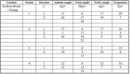
Chapter 2 Table 1: Capture information for Jess Dam 21 Table 2: Capture information for Kedron Brook at Grange. 22 Table 3: Capture information for Kedron brook at Keperra. 22

Table 4: Capture information for Samford. 23

Table 5: Capture information for Sherwood arboretum. 23 Table 6: Capture information for Tabragalba lagoon. 23 Table 7: Model selection weights for alternative closed

mark-recapture models, as calculated by program CAPTURE.

24

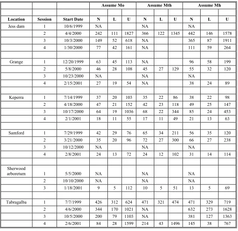
Table 8: Population size estimates (N) under three models for each location by mark-recapture session.

25

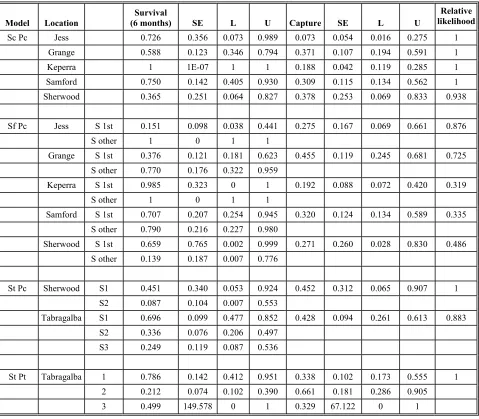
Table 9: Survival rate and catchability estimates for each

location under plausible models. 26

Table 10: Results of GROTAG analysis 27

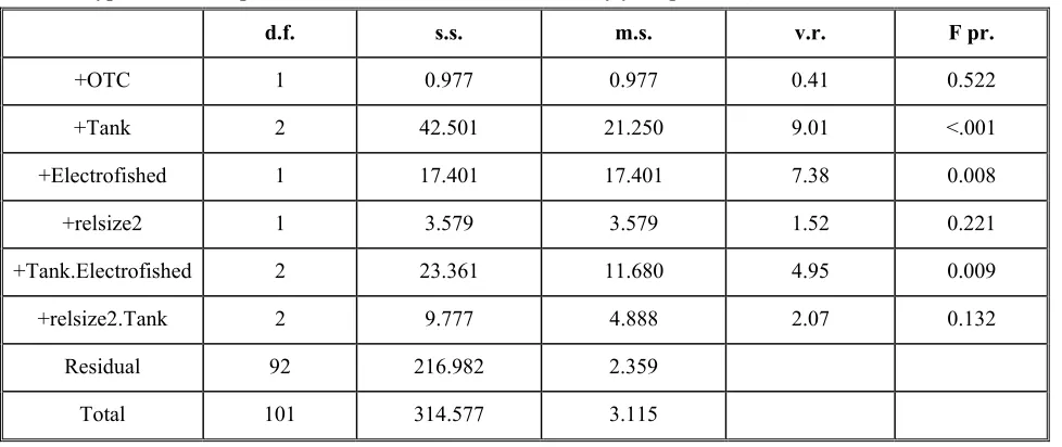
Chapter 3 Table 1: Accumulated analysis of variance table for growth during period 1, based on type 3 sums of squares.

34

Table 2: Estimated mean values for growth showing the interaction between electrofishing and OTC during the first growth period.

34

Table 3: Estimated mean values of growth showing the interaction between release size and tank during the first growth period.

35

Table 4: Accumulated analysis of variance table for growth during period 2, based on type 3 sums of squares.

35

Table 5: Estimated mean values of growth showing the effect of electrofishing and variation between tanks during the second growth period.

36

Table 6: Accumulated analysis of variance table for growth during period 3, based on type 3 sums of squares. Growth has been transformed by y = sqrt(x+12.5).

36

Table 7: Estimated mean values of growth showing the effect of electrofishing during the third growth period, with variation between tanks.

36

Chapter 4 Table 1: Position of OTC mark relative to nearest check in 81 tank held eels and estimated time of check formation.

49

Table 2: Number of subsequent check marks following

check nearest to OTC mark in 81 tank held eels. 50 Table 3: Position of OTC mark relative to nearest check in

marked-recaptured wild eels with estimated time of check formation and counts of observed subsequent checks formed compared with number of subsequent checks expected to form.

51

Table 4: Summary of ageing validation data for OTC marked wild caught eels (n = 35).

(8)

Chapter 5 Table 1: Prior distributions for model parameters. 67 Table 2: Posterior estimates for maturity, growth rate, and

mortality parameters, for silver eels collected in fishway sampling at Burnett River Barrage.

68

Table 3: Posterior parameter estimates for male, female, and undifferentiated eels caught during

fishery-independent electrofishing sampling in southeast Queensland.

75

Table 4: Posterior parameter estimates for male, female, and undifferentiated eels caught during

fishery-independent electrofishing sampling in New South Wales.

76

Table 5: Parameter estimates for Queensland age at length general linear model. Parameters for sites are differences compared to the reference site 1.

76

Table 6: Parameter estimates for NSW age at length general linear model. Parameters for sites are differences compared to the reference site CC11.

77

Chapter 6 Table 1:Model parameters for both sexes, and for both states unless stated otherwise.

85

Chapter 7 Table 1: Base levels of fishing mortality and management

constraints for each species, sex, and subpopulation. 105

Acknowledgements

(9)

Non-technical Summary

Principal Investigator: Dr Simon Hoyle

Address: Department of Primary Industries and Fisheries

PO Box 76

Deception Bay Qld 4508

Objectives:

1. Estimate population parameters required for a management model. These include survival, density, age structure, growth, age and size at maturity and at recruitment to the adult eel fishery. Estimate their variability among individuals in a range of habitats.

2. Develop a management population dynamics model and use it to investigate management

options.

3. Establish baseline data and sustainability indicators for long-term monitoring.

4. Assess the applicability of the above techniques to other eel fisheries in Australia, in

collaboration with NSW. Distribute developed tools via the Australia and New Zealand Eel Reference Group.

This project developed a user-friendly eel fishery management model to enable fisheries managers to investigate different management alternatives and their likely effects on trends in yield to the fishery and sustainable production of spawners.

In order to develop the model it was first necessary to validate whether eels from sub-tropical Queensland could be aged. The results of ageing validation experiments on both tank held eels and on tagged wild eels confirmed that long-finned eel stocks in sub-tropical Queensland could be aged reliably. Confirmation that eels could be aged, enabled estimation of

parameters such as age at maturity, growth, mortality and age at recruitment to the fishery. These parameters and others such as selectivity of the eel fishery and size at maturity data enabled development of an eel fishery management model.

Outcomes achieved: As a result of the development of the management model in this project the current management arrangements will not alter substantially in NSW and Queensland. Both states will continue to persist with areas closed to fishing. An agreement between DEH and DPI&F substantially recognises most of the findings and recommendations from this project, including using long-term monitoring CPUE data as an index of abundance and sustainability indicator and maintaining closures in freshwater riverine areas. Both DEH and DPI&F

acknowledge the importance of passage/trap and transport of elvers past artificial barriers and cost benefit options of different mechanisms are likely to be

investigated in the future.

(10)

Male eels in Queensland were observed to mature between 4 and 17 years and female eels between 5 and 39 years. Long-lived species such as eels that only spawn once are particularly vulnerable to overexploitation. Results of modelling suggest that long-finned eel stocks in Australia are best managed by having substantial areas closed to the fishery, to enable

maturation and escapement of spawning stock. The eel fisheries in Queensland and NSW are already essentially run along these lines, with freshwater riverine areas excluded from the fishery in both states.

Within Queensland the fishery is confined to impoundments and farm dams, and in NSW the fishery is concentrated in estuarine areas with some fishing also permitted in impoundments and farm dams. The results of the modelling from this project are likely to ensure the current management arrangements continue in both states, with no expansion of the fishery into freshwater riverine areas.

Results of modelling also suggest that spawner production and productivity of the fishery itself is likely to be improved through provision of elver passes or other means that will increase access of eels past barriers such as high dams and weirs. Improvement of fish passage is one area where current management arrangements of fisheries in both states could be improved, both for the benefit of the fisheries and for improved sustainability.

To monitor effectiveness of current management arrangements in sustaining production of spawners it has been recommended that the DPI&F freshwater fisheries long-term monitoring program be continued. An evaluation of this program showed that fishery independent CPUE data obtained from surveys of riverine areas was suitable for use as an index of abundance and sustainability indicator. Data collected by the program will be sufficient to detect changes between rivers and between years and is also able to be balanced for the influence of habitat parameters on CPUE.

(11)

Introduction

Background

This study supports the development and sustainability of the eel aquaculture industry, helps management of adult eel fisheries, and helps maintain the integrity of freshwater ecosystems in Queensland and throughout Australia. The research provides a management model for long-finned eels and the data to support the model in Queensland. It develops the data structures and analysis protocols to allow the model to be distributed and used for all Australia’s eel stocks, both short-finned and long-finned. The research also develops methodology and data structures for a fishery-independent sustainability indicator suitable for eel stocks throughout Australia, and collects baseline data for monitoring sustainability in Queensland.

The proposal was developed through discussions with the eel aquaculture industry and adult eel fishery representatives, glass eel researchers, and international eel experts. It arose from a perception of great potential risks of fishery collapse and very little knowledge of the long-finned eel. Perceptions were supported by preliminary population modelling work. The project had the support of the Queensland Fishery Service and industry groups. We consulted with the Freshwater Management Advisory Committee and eel aquaculturists. We also consulted with Drs Rick Fletcher, Bruce Pease, and Kevin Rowling of New South Wales Fisheries, who carried out a complementary and collaborative research program for New South Wales.

There are four species of Anguillid eel in Australia, of which two are common: the long-finned eel (Anguilla reinhardtii Steindachner, 1867) and one of the three short-long-finned species (A. australis australis Richardson, 1941). Eels are catadromous, migrating huge distances to spawn. Australian long-finned eels are thought to spawn in the Coral Sea. The East

Australian Current carries the larvae down the coast, where they metamorphose and enter estuaries anywhere from Cape York to Tasmania. In general, female eels grow larger and mature much later than males, and are found more often in the upper catchment than in estuaries. Males are seldom found outside brackish and estuarine areas but are known to occur in freshwater even in upstream areas.

Industry size and potential

Glass eel fisheries support a high value aquaculture industry worth well over $1 billion in Asia and Europe. Japan alone consumed over 100 000 tonnes of eel in 1996, and Europe uses about 25 000 tonnes per year. The growth of the Chinese and other Asian economies, where eel products have high value as a prestige food item, suggests that the value of this industry will continue to increase.

At the same time, supplies of glass eels from traditional sources in Asia and Europe are declining. Since the early 1980s German catches have dropped by 90 per cent and French by 86 per cent American, Taiwanese and Japanese eel supplies have also dropped substantially. There are now severe shortfalls in domestic supplies of glass eels in Japan and Taiwan, leading to very high prices and the rapid development of additional fisheries in, for example, the USA (New York Times, 16/2/1997). Catches there have also fallen. These drastic

(12)

Queensland is well placed to take advantage of this opportunity. The two main species of glass eels caught in our waters (Anguilla australis and A. reinhardtii) have good aquaculture potential and market acceptance. A. australis is potentially well accepted in the Japanese and Taiwanese markets, and A. reinhardtii in the Chinese market (Manhattan Industries, personal communication). An eel aquaculture industry is currently developing in Queensland, with a multi-million dollar facility recently completed in south-eastern Queensland. Other states also have multi-million dollar facilities. The industry was supported by an FRDC-funded project to identify the current status of and availability of glass eel supplies. An adult fishery also exists in Queensland, though its continued existence is under threat. The fishery has recently declined dramatically, apparently due to depletion of stocks in available waterways.

The Girramay, Gulmay and Jirrbal people traditionally harvest eels from the Tully-Murray area of Queensland by hook and line and basket traps. The Jumbin community (Girramay people) have expressed concerns about a reduction in eel catches on the Murray floodplain. This may be attributed to loss of wetland habitat. Nevertheless, commercial harvest of eels is also of concern to these people and the QFMA recommended that traditional use of eel resources needs to be considered in future management arrangements for the eel fishery (QFMA 1996).

Sustainability

The aquaculture industry depends on a continuing supply of glass eels. The FRDC glass eel project addressed supply identification and industry development, but did not address the overall sustainability of this very vulnerable resource. The growing value of eel products poses a serious threat to wild adult eel populations, which are the source of the glass eels. Adult eel fisheries have already declined in Queensland and New South Wales. High prices for adult eel products have encouraged expansion of the adult fishery into new areas as well as glass eel fishing, so the populations are doubly threatened. The risks involved are clear both from both the international declines, and the demonstrated ability of Queensland fishers to quickly deplete adult stocks (QFMA 1996) in the areas they fish.

Any fishing of adult eels has the potential to affect the glass eel supply. Eels are peculiarly vulnerable to fishing because of their unusual life history. Eels are very different from other fish, and cannot be managed in the same way. They have a very long generation time (approximately 20 years for Victorian shortfinned eels A. australis females, though up to 93 years has been documented for New Zealand longfinned eels A. dieffenbachii (Jellyman 1995)), low natural mortality, and all fishing occurs before breeding. Preliminary modelling suggested that even a low fishing mortality of 0.1 may reduce the number of female spawners produced from a stock to 23% of unfished levels. Since much of the fishery’s potential value is generated by spawning females, the risks are clear. These estimates are based on data for

A. australis in Victoria. Available evidence suggested the reduction may be more severe for

A. reinhardtii.

(13)

leading to poor recruitment, but given the longevity and catchability of eels, overfishing compounded by poor recruitment is possible. Catches of longfinneds in New South Wales have declined by 50% initially but have stabilised since the late 1990s.

The Queensland and NSW fisheries are very different. The Queensland fishery has operated mainly on females in fresh impounded waters, while the New South Wales fishery operates mainly on males in estuarine areas, although there is also an impoundment fishery

component.

Research summary

Management of eel stocks requires a different paradigm from most other fisheries, due to their remarkable life history. Population modelling proposed in this project will provide a basis for sustainable management of eel stocks throughout Australia. The model or models will be adaptable for management of both eel species throughout Australia.

Very little is known about Queensland’s eel stocks. Important demographic factors such as survival rates, age at maturity, and growth rate have not been studied for either of the major species in Queensland. Research on long-finned eels elsewhere in Australia has been very limited. Such research is clearly essential for informed management. We propose research into demographic factors important for management modelling of the longfinned eel fishery in Queensland and throughout Australia. The research framework, including database structures and a strong statistical component, will provide a basis for work on other eel stocks.

Monitoring of adults can provide early warning of declines and an indication of future glass eel trends, with far lower variability than glass eel monitoring. This project will develop the methodology and a database for collecting, analysing and sharing information on adult eel status and resource sustainability. It will develop the database structures, sampling techniques and statistical models to be used in ongoing monitoring.

Need

The research provides a management model for longfinned eels, and the data to support the model in Queensland. Supporting data for NSW were supplied by a collaborative project in that state. The model will also be suitable for managing shortfin eels in Victoria, Tasmania, NSW and Queensland, given appropriate data. The research has also developed methodology for a fishery-independent sustainability indicator, which will similarly be useful for both longfinned and shortfinned eels.

(14)

The FRDC is supporting glass eel industry development. However, sustainability of glass and adult eel fishing is not yet being addressed. Internationally, eel fisheries have not been sustained. Glass eel supplies have collapsed in Europe, Asia, and North America.

Our preliminary modelling of Queensland eel stocks demonstrated two things. Firstly, fishing of adult eels can severely reduce the number of spawning females. This is backed up by evidence from New Zealand, where the Lake Ellesmere eel fishery has seen drastic declines in the number of (particularly female) spawners (Jellyman 1995). Thus some types of adult eel fishing may damage the glass eel fishery. On the other hand, reduced or redirected adult eel fishing may significantly enhance the glass eel fishery. A management model was required to provide insight into these issues. Modelling of this kind has not previously been published for eels, and interest has been expressed by international eel researchers.

Secondly, very little was known about longfinned eel demography and population structure, knowledge which is needed for informed management of eel stocks. Some very sparse demographic data come from New Zealand, Tasmania and Victoria, but even this is

compromised by eels’ great variability in growth and maturation rates between environments. Queensland may hold the majority of longfinned eel biomass in Australia, but no studies had been carried out either here or in NSW. Statistically sound fishery-independent techniques are required to estimate population structure and demography for all important sectors of the population, particularly females. Fishery-dependent techniques will not work in Queensland due to the decline of the fishery. Data from NSW will provide complementary information on males which, it was thought, are probably seldom found outside estuaries.

As the glass eel fishery develops and as demand for adult eels rises, information on the changing status of wild eel stocks will be required. A sustainability indicator can provide this. Such indicators are best developed as early as possible in the evolution of the fishery.

Eel life histories are complex and unique, and successful management requires a different approach from other fisheries. Successful management of glass and adult eel fisheries requires a management model supported by demographic and fishery-based data. It also requires a feedback mechanism in the form of a sustainability indicator. The proposed research will provide the first and develop methodology for the second.

Objectives

1. Estimate population parameters required for a management model. These include survival, density, age structure, growth, age and size at maturity and at recruitment to the adult eel fishery. Estimate their variability among individuals in a range of habitats.

2. Develop a management population dynamics model and use it to investigate management options.

3. Establish baseline data and sustainability indicators for long-term monitoring. 4. Assess the applicability of the above techniques to other eel fisheries in Australia,

(15)

Chapter 1: An index of abundance for adult eels

Simon Hoyle, Michael Hutchison and David Mayer

Abstract

The low catch rates in the four large dams surveyed suggest that densities of eels are too low in most dams for monitoring of reservoirs by electro fishing to be of much value in assessing trends in eels stocks in the region. The DPI&F long-term monitoring program (LTMP) was found to be a suitable method for evaluating trends in eel stocks in rivers. LTMP surveys can be used to generate an index of abundance for legal sized long finned eel stocks. Should downward trends be detected in electrofishing CPUE over several years, then such a decline could be used as an early warning signal. This could lead to activation of surveys along the lines of the south-east Queensland (SEQ) eel surveys. The SEQ eel surveys covered a wider range of habitats and were at a finer scale and may be more useful in confirming recruitment of smaller eels.

A number of environmental parameters were found to have a significant influence on river and stream catches of eels. The depth effect is most pronounced for small eels, with catches of small eels tending to be greater in shallow waters, including riffle habitats. Other habitat variables with significant positive effects on catch rates of both large and small eels were rocks and aquatic macrophytes. Large eels were found to be associated with snags (woody debris) and undercut banks.

Objective

Establish baseline data and sustainability indicators for long-term monitoring.

Introduction

Australian longfinned eels (Anguilla reinhardtii) are believed to belong to a single panmictic stock. Therefore the number of new recruits entering a river system in one part of eastern Australia (e.g. Southern NSW) depends on the number of spawners contributed from all other parts of the east coast, including SEQ. Monitoring for sustainability across the panmictic population should target recruitment of new eels into river systems across eastern Australia, and provide an index of

abundance of adult eels. Monitoring glass eel arrivals would be designed to pick up overall changes in the level of recruitment, due to for example, a decline in spawning biomass. Local changes at a representative sample of sites would be informative about overall changes in the panmictic

population. However, glass eel arrivals are weather-dependent (Chisnall et al., 2002), and extremely variable in space and time (Pease et al., 2003), particularly in Australian conditions of high rainfall variation. It is very difficult to monitor them at a level sufficient to detect long-term changes.

Monitoring adult eels is preferable for several reasons. Sampling to monitor river fauna is already underway in Queensland. Adult eels are quite easy to catch and their numbers are relatively stable on short time scales, due to their longevity. Long-term changes are therefore easier to detect. Such an index could also pick up local changes within rivers, which may occur as a result of the erection or removal of downstream barriers or other local factors such as changes to habitat condition or overfishing. Severe local impacts across a number of catchments could lead to eventual

panmictic declines in recruitment. Therefore being able to identify declines within a river system is also important.

Having an index of abundance monitoring system in place will assist in early detection of

(16)

Methods

This project evaluated two possible methods for long-term monitoring of eel stocks using an index of abundance. The first is the survey method developed for the current project for collection of eels for population age structure data. The second is the Queensland Fisheries Service’s Long-Term Monitoring Program for freshwater fish stocks.

Survey Methods: South-east Queensland eel surveys (this project)

Sampling concentrated on freshwater reaches since the females tended to concentrate in these areas. Female population dynamics are more sensitive to fishing and are more important to the

sustainability of glass eel and adult fisheries. Sampling was restricted to south-eastern Queensland, with Bundaberg the northern limit. Sampling was stratified into reaches in small streams, reaches in large streams, and impounded waters. Impounded waters included three sites on Wivenhoe dam (fished), three sites on Lenthalls Dam (fished) three sites in Enoggera Reservoir (unfished), and three sites at Tingalpa reservoir (unfished). In addition ten sites were selected in small streams that had not been fished (tributaries of the Albert, Logan, Coomera and South Pine Rivers), ten sites in larger unfished waterways (Albert, Logan, Coomera and South Pine Rivers), and ten sites in larger fished waterways (Mary and Caboolture Rivers, Tinana Creek). Sites on two of the unfished streams (Albert and Logan Rivers) had glass eel fishing at the mouth, and glass eel sampling occurring under FRDC project 97/312. At all sites both longfinned and shortfinned eels were sampled. Locations of sampling sites are shown in Figure 1.

Within these sites, transects were chosen as randomly as practicable. Each waterway was divided into 10 by 10 km blocks, and three blocks selected at random. Within these blocks, all suitable access points were determined, and one of these was randomly selected as an appropriate starting point.

For each site distance from the sea and existence of barriers to migration such as barrages were recorded. At a 5 metre shot level (see below), depth and habitat variables were recorded. Habitat variables recorded included gross habitat type (pool, riffle, run, cascade and backwater), depth and width of stream. Other habitat features were scored on a semi-quantitative or categorical five point system of zero to four. Zero denoted the habitat feature was absent, whereas scores from 1 through to 4 denoted a range of importance from minor to major. Habitat features scored in this way were snags or large woody debris, undercut banks, aquatic macrophytes, aquatic grasses, rocks,

overhanging vegetation, canopy cover, and side creeks.

At each site the size structure of the population was investigated by electrofishing along one hundred-metre transects. Each transect was broken up into 5 metre shots and fished from

downstream to upstream. In large streams each of three transects was electrofished as separate 5 metre shots on each bank.

On small streams six transects were fished in series with both banks included in a single shot. In impoundments 5 metre shots were conducted along a randomly selected shoreline. Up to six transects were run in each impoundment.

All sites were fished in two passes. In small streams and shallow riffle habitats backpack

(17)

Figure 1: South-east Queensland eel survey age structure and index of abundance sampling sites.

Survey methods: Queensland Fisheries Service’s Long-Term Monitoring Program (LTMP) The Queensland Fisheries Service Long-term monitoring program monitors ten river systems in Queensland by boat electrofishing on an annual basis. Six of the rivers are within the distribution of longfinned eels. Three are located in the southeast (Noosa, Albert-Logan and Mary River systems) and three are located in the tropical north (Herbert, Johnstone and Daintree Rivers). Eels comprise one of the target species for surveys within these rivers. Full descriptions of the methodology used for the long-term monitoring program are found in Hutchison et al. (2004). The methods are summarised here. On each of the rivers seven fixed reaches are sampled by electrofishing boat. Initial selection of reaches was random. Within each reach, six–50 metre sites or shots are selected randomly each year. Shot sites extend 15 metres from the bank. These sites are fished using

standardised electrofishing boat manoeuvres involving pre-determined application of electrofishing power by time and space within the site. Numbers and total length of all eels captured is recorded at each site. At each of these 50 metre sites various habitat parameters are also recorded. Protocol for recording for habitat details was adapted from the system used by Russell et al (2000). Habitat details recorded included pH, conductivity (ms/sec), oxygen (mg/L), turbidity (NTU and Secchi depth cm), water temperature (°C), maximum depth (m), stream width (m), current velocity, bottom substrate, in-stream snags, rocks, grasses, leaf-litter, aquatic macrophytes, emergent vegetation, riparian vegetation width (m), riparian continuity and composition, canopy cover, cover, and index of disturbance.

(18)

the per cent composition of trees, grasses and bare ground. In-stream habitat features such as rocks, snags, aquatic macrophytes, and leaf litter are scored from 0 to 5 based on the surface area of the shot zone each of these features occupies. A score 0 indicates the feature is absent, 1 = <50 m2, 2 = 50–100 m2, 3 = >100 m2, 4 = >150 m2 and 5 = >200 m2. Overhead or canopy cover was scored in the same way. Undercut banks and emergent vegetation (reeds, rushes) were also scored from 0 to 5. In this case the score relates to the length of shoreline or bank of this type. If the feature is absent it is scored 0. A score of 1 = ≤10 m, 2 = ≤20 m, 3 = ≤30 m, 4 = ≤40 m and 5 = ≤50 m. Bottom substrate was classed as boulder/cobble, cobble/gravel, sand and fine material. Each of these substrates was scored from 1 to 4, with 1 being the most abundant and 4 the least abundant.

Statistical Methods — south-east Queensland eel surveys

The survey design generally consisted of 20 shots within each site, at one sampling date. At each site, two successive samples were conducted, with the eels from the first 20 shots not being returned prior to the second shots being taken (this contributed better independence between samples). The total number of shots was 230 in dams and reservoirs, and 1270 in rivers and streams. True spatial or temporal replication of sites was minimal (6-degrees-of-freedom). However, the environmental variables of interest were measured within-sites, so shots is the appropriate experimental unit for fitting these terms, provided that any spatial autocorrelations amongst the residuals are low.

‘Dam’ and ‘other’ (riverine) sites clearly had different types of environmental variables, as well as different catch rates. Hence, these data sets were analysed separately. Sites with zero captures (over all times and shots), and hence zero deviances, were noted and excluded from these analyses.

A Poisson generalised linear model (GLM) with log link (McCullagh and Nelder, 1989) was used to model the numbers of eels, via GenStat (2000) — separately for total, ‘large’ (>300 mm), and ‘small’ (≤300mm) eels. ‘Sample’ was fitted first (to estimate the fish-down effect), and was always significant (P<0.01). Then, step-forward selection of main effects was employed to arrive at a model for total eels where all environmental effects were significant (at P<0.05, and using the theoretical dispersion coefficient of one). Next, the ‘site’ term was checked for significance, to see whether the observed differences in eel numbers had been adequately explained by the

environmental variables. Finally, all two-way interactions between these significant effects were tested for significance, and the tabulated means were checked for biological meaning. Residuals from this model were examined for spatial and temporal (between-samples) correlations, and adjusted means for each effect were tabulated.

A follow-up comparison between rivers with different fishing pressures (none, fished, glass-eel harvests) was also undertaken. Because this factor was totally aliased with 'site' (in that sites were nested within this classification), this ‘fishing pressure’ term was fitted as a 2-degrees-of-freedom contrast within the ‘site’ coefficients.

Hierarchical generalised linear models (Lee and Nelder, 2001) were also investigated for the riverine data (total eels), using GenStat (2000). These HGLM’s extend generalised linear models to allow the inclusion of an extra random term in this case, the top (but minimally estimable) level of replication. This term was modelled as a gamma distribution with the log link (Nelder, pers. comm., 2001). The Choleski method for adjusting the likelihood profile, and first-order Laplace

(19)

Statistical methods: LTMP surveys

A Poisson generalised linear model (GLM) with log link (McCullagh and Nelder, 1989) was used to model the numbers of eels, via GenStat (2000) separately for total, ‘large’ (>300 mm), and ‘small’ (≤300 mm) eels. Step-forward selection of main effects was employed to arrive at a model for total eels where all environmental effects were significant (at P<0.05, and with the more

conservative approach of using the fitted dispersion coefficient). Next, the ‘river’ term was checked for significance, to see whether the observed differences in eel numbers had been adequately

explained by the environmental variables. Finally, the ‘year’ term and ‘year by river’ interactions were added, to test for variations in the annual patterns between the rivers. Residuals from this model were examined for spatial correlations (between-shots, as there were generally six shots per sampling date), and adjusted means for each effect were tabulated.

Results

South-east Queensland eel surveys

In the hierarchical generalised linear model, the fitted deviance for the additional (top-level) replication was less than that of the full model. Hence, this HGLM defaulted back to the Poisson GLM. This pattern was also noted in an approximate split-plot GLM of ln(Y+1)-transformed data using the Normal distribution, where the top-level residual mean square was less than that of the main model. This further justifies using shots as the experimental units in the final Poisson GLM.

Dams Data

No eels were caught in Tingalpa Reservoir or Wivenhoe Dam. A total of 34 eels were caught at four sites in Enoggera Reservoir (3) and Lenthalls Dam (31). These were all classified as large; no smalls were captured.

Aquatic macrophyte was the only environmental variable to be significantly associated with capture rates. Unfortunately, it was highly aliased with site (also significant), making interpretation of these patterns (Table A1) somewhat difficult. This model explained 55% of the total deviance, and both the temporal and lag-one spatial correlations between model residuals (r = –0.15 and –0.08,

respectively) were not significant (P>0.05). The fish-down effect was quite pronounced, with 76 per cent being captured in the first sample (adjust overall mean of 0.413, versus 0.127 for the second sample). The model was under-dispersed with a residual mean deviance of 0.61 — this indicates that these large eels were distributed more evenly than was expected by the random Poisson model, i.e., statistically, they displayed territorial behaviour.

Table A1. Adjusted average capture rates of large eels in dams, by site and type of aquatic macrophyte.

Dam Site

number macrophyteAquatic Number of shots Average no. eels (/shot) Standard error

Enoggera Reservoir 1 4 20 0.10 0.07

2 4 20 0.05 0.05

Lenthalls Dam 4 3 4 0.00 0.00

4 4 16 0.31 0.14

5 0 14 1.21 0.29

(20)

Riverine Data

Only one site had zero captures Emery Bridge, on the Mary River, with 40 shots. For the other sites, table A2 summarises the goodness of fit for the Poisson GLMs. In every model, ‘site’ was a

significant contributor after the environmental variables had been screened, indicating that the site differences could not be totally explained by these attributes. Tables A3 to A9 list the adjusted means for the significant terms in these models, namely depth, type of stream, rocks category, aquatic macrophyte, snags, undercut bank and overhanging vegetation. Interestingly, the non-significant variables were turbidity (Secchi method), width of stream (likely to be correlated with depth), grass, and canopy cover (likely to be correlated with overhanging vegetation). These either had no association with catch rates, or alternately may be correlated with other variables already in the model (and hence had no further statistical contribution). Tables A10 and A11 give the adjusted means for the sample and site effects, respectively.

Tables A12 and A13 show the adjusted means and raw means for the follow up comparison between rivers with different fishing pressures. In no cases was fishing pressure significant (P>0.05), indicating that the observed ‘site’ differences could not be attributed to differing fishing pressures. However, the fitted means are of interest in that the mean values for fished sites are lower than for those of fished sites, with the signal being quite strong (magnitude of 10) and close to significant for small eels, but the pronounced background variation means this is not a significant signal (p = 0.07).

Table A2. Goodness of fit of the Poisson GLMs for eel captures.

Parameter Total count Large eels Small eels

Residual mean deviance 0.80 0.53 0.55

Deviance explained (%) 67.8 41.9 73.0

Spatial autocorrelation (r) 0.16 0.06 0.17

Temporal correlation (r) 0.12 0.14 0.07

Table A3. Adjusted average capture rates (per shot), by depth.

Depth Total count Large eels Small eels

1 0.82 0.19 0.58

10 0.73 0.19 0.47 50 0.43 0.19 0.18 100 0.22 0.19 0.05 150 0.12 0.19 0.02 200 0.06 0.20 0.00 250 0.03 0.20 0.00

Table A4. Adjusted average capture rates (per shot), by stream physical habitat type.

Stream type No. of shots Total count Large eels Small eels

Pool 560 0.30 0.16 0.11

Riffle 180 0.60 0.22 0.24

Run 471 0.43 0.20 0.16

Cascade 8 0.93 0.71 0.33

(21)

Table A5. Adjusted average capture rates (per shot), by rocks.

Rocks No. of shots Total count Large eels Small eels

0 450 0.24 0.12 0.08 1 195 0.26 0.13 0.11 2 153 0.47 0.22 0.17 3 253 0.46 0.18 0.19 4 208 0.74 0.38 0.28

Table A6. Adjusted average capture rates (per shot), by aquatic macrophyte.

Aquatic macrophyte

No. of shots Total count Large eels Small eels

0 1107 0.37 0.19 0.14

1 85 0.41 0.18 0.14

2 38 0.88 0.21 0.32

3&4 29 0.95 0.31 0.43

Table A7. Adjusted average capture rates (per shot), by snags.

Snags No. of shots Total count Large eels Small eels

0 459 0.41 0.17 0.16 1 345 0.33 0.18 0.11 2 233 0.51 0.26 0.18 3 109 0.52 0.27 0.17 4 113 0.17 0.05 0.19

Table A8. Adjusted average capture rates (per shot), by undercut bank.

Undercut

bank No. of shots Total count Large eels Small eels

0 701 0.37 0.14 0.17

1 348 0.45 0.28 0.15

2 153 0.50 0.24 0.17

3 57 0.18 0.16 0.03

Table A9. Adjusted average capture rates (per shot), by overhanging vegetation.

Overhanging vegetation

No. of shots Total count Large eels Small eels

0 469 0.49 0.21 0.22 1 549 0.36 0.20 0.12 2 225 0.33 0.15 0.12

3 16 0.17 0.00 0.11

Table A10. Adjusted average capture rates (per shot), by sample.

Sample No. of shots Total count Large eels Small eels

1 670 0.51 0.26 0.19 2 589 0.28 0.12 0.11

(22)

Table A11. Raw and adjusted average capture rates (per shot), by river and site.

River Site within river No. shots

Total count

Large eels Small eels

raw adj. raw adj. raw adj.

Albert (main) Chardons Bridge 80 0.01 0.12 0.01 0.06 0.00 0.00 Darlington Park 40 6.40 1.93 1.63 1.15 4.78 0.78

Nindooinbah 40 1.33 0.96 0.25 0.22 1.08 0.68

Albert (tribs.) Canungra Creek 40 0.20 1.39 0.08 0.39 0.13 0.46 Cedar Creek 40 0.48 0.34 0.13 0.12 0.35 0.23 Sandy Creek (Albert) 20 0.05 0.04 0.05 0.08 0.00 0.00

Caboolture Site 1 40 0.15 0.07 0.10 0.11 0.05 0.01

Site 2 40 0.15 0.13 0.10 0.12 0.05 0.03

Site 3 40 0.40 0.24 0.28 0.21 0.13 0.06

Site 4 40 0.70 0.25 0.43 0.21 0.28 0.08

Coomera (main) Beechmont Rd 40 4.73 1.59 1.25 0.83 3.48 0.75 Clagiraba Road 43 1.33 0.79 0.19 0.18 1.14 0.43 Guanaba Creek Road 40 0.23 0.52 0.15 0.19 0.08 0.30 Coomera (tribs.) Guanaba Creek 40 0.43 0.18 0.08 0.06 0.35 0.12

Prices Creek 42 0.29 0.13 0.19 0.13 0.10 0.03 Wongawallan Creek 40 0.28 0.10 0.13 0.06 0.15 0.05 Logan (main) Cusack Lane 80 0.10 0.17 0.04 0.06 0.06 0.10

Williams Bridge 20 0.15 0.17 0.15 0.19 0.00 0.00 Logan (tribs.) Cannon Creek 40 0.10 0.07 0.05 0.08 0.05 0.02

Sandy Creek (Logan) 40 0.25 0.21 0.13 0.18 0.13 0.06

Mary Kenilworth 20 0.25 0.24 0.25 0.40 0.00 0.00

Moy Pocket 80 0.09 0.60 0.09 0.14 0.00 0.00

South Pine (main) Drapers Crossing 42 0.29 0.22 0.19 0.15 0.10 0.09 Morrisons Crossing 48 0.67 0.25 0.27 0.17 0.40 0.09 South Pine (tribs.) Albany Creek 40 0.10 0.19 0.08 0.12 0.03 0.05

Samford Creek 44 0.27 0.26 0.07 0.12 0.20 0.13 Tinana Creek Missings 80 0.03 0.16 0.03 0.04 0.00 0.00

Wilsons Pocket Road 60 0.07 0.05 0.05 0.05 0.02 0.01

Table A12. Adjusted average capture rates (per shot), by fishing pressure.

Pressure No. of shots Total count Large eels Small eels

Fished 440 0.22 0.16 0.02

Glass-eel harvest 340 0.54 0.25 0.23

Unfished 859 0.42 0.20 0.20

Table A13. Raw average capture rates (per shot), by fishing pressure.

Pressure No. of shots Total count Large eels Small eels

Fished 440 0.23 0.17 0.07

Glass-eel harvest 340 0.91 0.25 0.66

Unfished 859 0.86 0.26 0.60

LTMP eel surveys

(23)

for the total and large eels models, but not in the small eels analysis (but was retained here, for consistency). Tables C2 to C9 list the adjusted means for the significant terms in these models, namely river, river by year, water velocity, snags, voltage, rocks category, level of disturbance, and aquatic macrophyte. The non-significant variables were year; depth, width, water level, riparian continuity and tidality of the river; amperage and gain of electrofishing (correlated with voltage); width of the riparian vegetation; percentage of trees, grasses or no vegetation; canopy cover; overhanging vegetation; type of emergent vegetation; leaf litter; undercut bank; and substrate type. These either had no association with catch rates, or alternately may be correlated with other

variables already in the model (and hence had no further statistical contribution).

Table C1. Goodness of fit of the Poisson GLMs for eel captures.

Parameter Total count Large eels Small eels

Residual mean deviance 1.29 1.07 0.70

Deviance explained (%) 35 35 21

Spatial autocorrelation (r) 0.11 0.06 0.12

Table C2. Raw and adjusted (modelled) average capture rates (per shot), by rivers.

River No. Total count Large eels Small eels

shots raw adjusted raw adjusted raw adjusted

Daintree 84 2.19 1.64 1.74 1.30 0.45 0.32 Herbert 60 1.63 1.72 1.13 1.23 0.50 0.48 Johnstone 84 1.08 0.82 0.76 0.57 0.32 0.25 Logan 84 0.60 0.77 0.40 0.52 0.19 0.26 Mary 84 0.64 0.75 0.48 0.56 0.17 0.20 Noosa 84 0.16 0.21 0.14 0.18 0.01 0.02

Table C3. Adjusted average capture rates (per shot), for years by rivers.

River Total count Large eels Small eels

2000 2001 2000 2001 2000 2001

Daintree 1.98 1.32 1.62 1.00 0.34 0.31

Herbert 1.81 1.64 1.36 1.10 0.43 0.53

Johnstone 0.94 0.71 0.65 0.50 0.29 0.21

Logan 0.66 0.88 0.47 0.57 0.20 0.33

Mary 0.39 1.08 0.28 0.81 0.11 0.28

Noosa 0.17 0.24 0.17 0.19 0.00 0.05

Table C4. Adjusted average capture rates (per shot), by water velocity.

Water velocity No. of shots Total count Large eels Small eels

High 9 0.48 0.23 0.26

Moderate 388 1.27 0.95 0.23

Low 81 0.90 0.67 0.31

Table C5. Adjusted average capture rates (per shot), by snags.

Snags No. of shots Total count Large eels Small eels

0 143 0.63 0.41 0.22 1 263 1.05 0.79 0.26

2 52 1.15 0.94 0.22

3 13 1.34 0.96 0.36

(24)

Table C6. Adjusted average capture rates (per shot), by voltage.

Voltage Total count Large eels Small eels

320 0.69 0.51 0.17

340 0.70 0.52 0.18

500 0.79 0.59 0.20

700 0.92 0.68 0.24

1000 1.15 0.86 0.30

Table C7. Adjusted average capture rates (per shot), by rocks category.

Rocks No. of shots Total count Large eels Small eels

0 339 0.85 0.63 0.22

1 70 1.11 0.81 0.29

2&3&4 30 1.24 0.98 0.26

5 41 1.33 0.95 0.37

Table C8. Adjusted average capture rates (per shot), by level of disturbance.

Disturbance No. of shots Total count Large eels Small eels

Extreme 21 1.52 1.22 0.30

High 132 1.08 0.78 0.29

Moderate 101 0.80 0.60 0.21

Low 89 0.98 0.71 0.27

Undisturbed 133 0.84 0.63 0.21

Table C9. Adjusted average capture rates (per shot), by type of aquatic macrophyte. Aquatic

macrophyte No. of shots Total count Large eels Small eels

0 361 0.90 0.69 0.21

1&2 105 1.06 0.73 0.34

3&4&5 14 1.57 1.10 0.48

Discussion

South-east Queensland eel survey

The low catch rates in the four large dams surveyed suggest that densities of eels are too low in most dams for monitoring of reservoirs by electrofishing to be of much value in assessing trends in eels stocks in the region. Although commercial landings suggest fished dams have been depleted of eel stocks (QFS C fish database), both a fished dam (Wivenhoe) and an unfished dam (Tingalpa) had zero captures, suggesting that factors in addition to fishing could be involved in the low catch rates. One trend identified was lower catches in dense macrophyte beds. In reservoirs in Queensland macrophyte beds can extend out into six metres of water and reach from the bottom to the surface. At this depth efficiency of electrofishing is compromised. Although eels might use these weed beds, the depth of the beds can make detection of stunned eels and netting of observed eels difficult. It is possible that eels were present in the dams at deeper levels, but beyond the range of the

electrofisher.

(25)

New Zealand longfinned eels, but flows over low weirs are much more likely to be sustained in New Zealand than they are in South-east Queensland. In New Zealand high dams are known to exclude or severely reduce recruitment of eels. For example no eels were found in Lake

Mahinerangi, a New Zealand hydro-electric storage (Allibone, 1999).

Elvers and glass eels leaving the water to bypass weirs are more at risk of predation. Opportunities for elvers and glass eels to migrate up dam walls are limited to those times when water is spilling over the dam, creating damp surfaces, and possibly also to rainfall events which create damp

surfaces. Failure to migrate upstream and mortality from predation can be expected to increase with increasing dam height. Higher dams also tend to spill less often. Thus replenishment of dam stocks following fishing activities or loss of downstream migrants can be compromised. Lenthalls dam spills in most years during summer and this may explain the better catches from this dam compared to the others sampled. No small eels (<300mm) were caught in any of the dams suggesting

recruitment must have been poor in recent years or that small eels were not using the lacustrine habitats sampled by electrofishing.

A number of environmental parameters were found to have a significant influence on river and stream catches of eels. The first of these is depth. The depth effect is most pronounced for small eels, with catches tending to be greater in shallow waters. Jellyman et al., (2003) also noted that juveniles of both species of New Zealand eels preferred shallow water. Broad et al. (2001a) found a similar result for A. dieffenbachia, and reported that eels were significantly longer in pools than in riffles. In our study shallow waters generally corresponded to riffle habitats, cascades and

backwaters, where we observed large concentrations of juvenile eels (see Table A5). Use of these shallow areas may have afforded small eels some protection from predation by large eels and other predatory fishes. The depth effect was less marked for large eels, but there is a slight tendency for large eels to be more prevalent in deeper water. This includes deeper holes at the bottom of cascades.

Other habitat variables with significant positive effects on catch rates of both large and small eels were rocks and aquatic macrophytes. We conclude that eels take advantage of the cover provided by rocks and macrophytes in rivers and streams. The macrophyte result contrasts with that of dams, but macrophyte beds in rivers and streams were shallower and easier to sample by electrofishing than those in dams. Jellyman et al. (2003) noted that large (>500mm) eels in New Zealand were strongly associated with cover, which included undercut banks, weed and in-stream debris.

(26)

In contrast, overhanging vegetation was negatively associated with catch rates of both small and large eels. This may in part be related to eels being more visible in areas without overhanging vegetation and more difficult to dip-net from under overhanging vegetation, but there does appear to be a real effect. It is generally more disturbed areas that lack overhanging vegetation. These same areas may also favour macrophyte growth, with which eels have been positively associated in this study. Macrophyte abundance was weakly negatively correlated with overhanging vegetation.

The SEQ eel surveys were one-off samples, so no comparison could be made between years. However, between-site differences were detected which could not be explained by the evaluated environmental parameters alone. If between-site differences can be detected, then the data should be sensitive enough to pick up a signal if significant changes in density occur through time.

It is interesting that no significant difference in eel catch rates was detected between sites in fished and unfished catchments, although the variability within both fished and unfished rivers, and therefore the power of this type of test, was such that even a large difference would have been difficult to detect. The large difference observed (lower in fished catchments) was not statistically significant. Fishing impacts may have been minimal compared to other effects in the rivers, since commercial fishing is restricted to weir pools within the fished rivers. Tributary streams and

unimpounded sections remain unfished. Movement of eels between fished and unfished areas of the rivers is likely, and this could mask any local impacts. The proportion of the sampled rivers that is fished is probably not large enough to significantly affect the river system as a whole. Glass eel harvest was not observed to affect abundance of large or small eels, though again the power of this test was low. Current levels of glass eel harvest may be below those where density dependent impacts on recruitment might occur. Enough glass eels may be escaping capture for density independent recruitment to still take place.

LTMP eel survey data

The results from this data are largely consistent with the results of the SEQ eel survey. A key

difference between the two sets of data is that habitat variables in the SEQ eel survey were collected at a 5 m shot level, whilst the LTMP data is collected at a 50 m shot level. The other key difference is that the LTMP program data comes entirely from the main stream of key rivers, whereas the SEQ eel surveys also included small tributary stream sites. The SEQ surveys used both backpack and boat mounted electrofishing, whereas the LTMP data is restricted to boat mounted electrofishing and areas deep enough for boating. Therefore it is not surprising that depth was a significant variable in the SEQ eel survey data, but not significant in the LTMP data, as the range of depths sampled by the latter method were more restricted.

Snags, rocks and aquatic macrophytes were all found to be significant influences on LTMP eel catch rates. The same variables were identified as significant in the SEQ eel survey data. All three variables were positively associated with LTMP total eel catch rates. In the case of small eels the effect of snags was less than that for large eels, and adjusted mean captures of small eels were lower in the most abundant snag categories (4&5) than in the preceding moderate (3) category. A similar result was noted with the SEQ eel survey data. In contrast to this result, Broad et al. (2001b) found the New Zealand species of longfinned eel A. dieffenbachii to be negatively associated with wood debris in the Taieri River. For modelled LTMP data, adjusted mean recaptures of large eels

increased with abundance of snag cover and captures of both large and small eels increased with increasing rocks and macrophytes. This is also consistent with SEQ eel survey results.

(27)

relationship with overhanging vegetation. A number of the variables not selected by the GLM as significant for the LTMP eel data may have been correlated with the index of disturbance, for example, riparian continuity and width and overhanging vegetation. Similarly in New Zealand, Broad et al. (2001b) found A. dieffenbachii to be more abundant in catchments with pasture, than in catchments with native forest. That eels are favoured by disturbance is an interesting result. One of us (M.H.) has observed A. reinhardtii in urban drains where no other native fish survive. Thus eels appear to be more tolerant of poor water quality and disturbed habitats than most other native fish species. Reduced competition with, and predation by other fish species in disturbed areas may favour eels. Eel catch rates were also positively associated with voltage settings used during electrofishing. Voltages were set higher by operators in low conductivity conditions and were set lower in higher conductivity conditions in an effort to standardise power outputs. The lowest conductivities were in the northern rivers and these rivers tended to have higher catch rates of eels. Whether voltage was a real effect on catch rates or an artefact of where sampling took place is open to conjecture.

The most important result with the LTMP data is that in every model, ‘river’ was a significant contributor after the environmental variables had been screened, and the ‘year by river’ interaction was significant for the total and large eels models. This suggests that the LTMP eel data should be suitable for monitoring trends in stocks of large eels, between rivers and between years. The LTMP sampling is mainly confined to river pools and does not sample shallower habitats that tend to be favoured by smaller eels (see SEQ eel survey data). This is possibly why these data were unable to detect between-river or between-year differences in small eel numbers. Nevertheless large eel numbers give some indication of the abundance of potential spawners and this is an important consideration when managing eel stocks.

The LTMP eels surveys have been set up to monitor a range of freshwater fish stocks in

Queensland. These surveys are planned to continue into the foreseeable future. The analysis of the LTMP data suggests that these surveys are suitable for detecting changes in abundance of large eels (i.e. those potentially available to the adult eel fishery) and total eel numbers. Therefore LTMP surveys can be used to generate an index of abundance for legal sized longfinned eel stocks. Should downward trends be detected in electrofishing CPUE over several years, then such a decline could be used as an early warning signal. This could lead to activation of surveys along the lines of the SEQ eel surveys. The SEQ eel surveys covered a wider range of habitats and were at a finer scale and may be more useful in confirming recruitment of smaller eels. These studies may also help confirm whether declining large eel stocks are related to reduced recruitment of small eels or other factors that are impacting on larger eel size classes.

Identification of habitat factors significantly influencing catch rates in both the LTMP and the SEQ eel surveys is interesting. One of the main reasons for identifying such habitat factors was to

(28)

Hoyle and Jellyman (2002) suggested New Zealand longfinned eels need catchment reserves to provide for sufficient spawner escapement. Graynoth and Niven (2004 in press) developed a GIS system to estimate the proportion of longfinned eel biomass in New Zealand’s West Coast and Southland that exists in areas not currently fished. This macro-scale GIS habitat based model uses mean annual flow and stream reach gradient as the key predictors of biomass distribution. The macro-scale habitat variables were selected in preference to micro-habitat variables such as water depths, velocities and substrates, as such detailed information was not available at a large geographical scale. Biomass was preferred over abundance indices as the density of large eels (i.e. eels >400 mm TL) was strongly correlated with biomass. Overall densities, on the other hand, were strongly influenced by the number of small eels. The number of large eels (potential

spawners) is more important when considering adequacy of reserves, thus predictors of biomass were useful for sustainable management of the fishery. There was also some evidence that biomass of small eels may increase following removal of large eels, due to improved density dependent survival. Thus biomass was a useful predictor of the potential of eel reserve locations.

The current habitat data collected for both the LTMP and the SEQ eel surveys has been at more of a micro-habitat level. For some of these (e.g. riffle, pool, backwater) it may be possible to estimate parameters remotely. It may also be possible to estimate density of large woody debris from air photos etc in the main stream of river systems. However macro-scale variables such as stream reach gradient, mean annual flow, elevation and stream order are more easily obtainable for entry into a broad regional GIS model. Whether these macro-variables will be as useful in an Australian context as in New Zealand as predictors of eel biomass remains unknown. Their potential should be

investigated.

If they are shown to have strong predictive capacity for either eel biomass or abundance of different size classes, then they could be used to develop a GIS model to assist with selection of eel

catchment reserves in eastern Australia.

The micro-habitat variables identified as important from the SEQ eel surveys and the LTMP could perhaps be incorporated into catchment or sub-catchment GIS models for eel stocks, although collection of such data would be difficult for GIS models covering larger geographical areas. Nevertheless the knowledge of important microhabitats gained from this current analysis could be useful information for rehabilitation or wetland creation works, where the aim is to favour either recruitment of small eels, supporting stocks of large eels or both. Certainly there is potential for such programs under a number of recent Commonwealth Government natural resource management funding initiatives.

Conclusions

1. Current densities of eels in large impoundments are too low for these locations to be suitable for long-term monitoring of eel stocks.

2. The existing LTMP for river eel stocks appears suitable for use as an index of abundance for large eels and total eel catch. Numbers of large eels are critical in terms of future potential spawners, and any downward trends in abundance could be used as an early warning for future spawner production.

3. There is no statistically significant evidence for a decline in eels in SEQ rivers that is attributable to either adult eel harvest or glass eel harvest. Nevertheless there was a non-significant trend for eel catch rates to be lower from sites in fished catchments.

(29)

5. If the LTMP detects declines in large eel or total eel abundance within a single river or across several rivers, then a SEQ style survey could be re-implemented to examine a broader range of habitat types (including those favoured by smaller eels) to better define at which stage of the eel life history losses are occurring.

6. The value of macro-habitat variables (e.g. mean annual flows, stream reach gradient) for

predicting the distribution of eel biomass in Australian catchments needs to be investigated. If these variables prove to be useful predictors, then they could be incorporated into a GIS system that could be developed for managing the eel fishery through appropriate distribution 7. of eel fishing reserves (see Chapter 6).

References

Allibone, R.M. (1999) Impoundments and introduction: their impacts on native fish of the upper Waipori River, New Zealand. Journal of the New Zealand Royal Society29(4), 291–299.

Chisnall, B.L., Jellyman. D.J., Bonnett, M.L. and Sykes, J.R. (2002) Spatial and temporal

variability in the length of glass eels (Anguilla spp.) in New Zealand. New Zealand Journal of Marine and Freshwater Researchi 36(1), 89–104.

Broad, T.L., Townsend, C.R., Closs, G.P. and Jellyman, D.J. (2001a) Microhabitat use by longfin eels in New Zealand streams with contrasting riparian vegetation. Journal of Fish Biology 59(5), 1385–1400.

Broad, T.L., Townsend, C.R., Arbuckle, C.J. and Jellyman, D.J. (2001b) A model to predict the presence of longfin eels in some New Zealand streams, with particular reference to riparian vegetation and elevation. Journal of Fish Biology 58(4), 1098–1112.

GenStat (2000) GenStat for Windows, Release 4.2, Fifth Edition. VSN International Ltd., Oxford.

Graynoth, E. and Niven, K. (2004) Longfinned female eel habitat in the West Coast and Southland. Department of Conservation, Science and Research Report (in press).

Hoyle, S.D. and Jellyman, D.J. (2002) Longfin eels need reserves: Modelling the impacts of commercial harvest on stocks of New Zealand eels. Marine and Freshwater Research 53, 887–895.

Hutchison, M., Jebreen, E., Helmke, S. and Lunow, C. (2004) Fisheries Long-term Monitoring Program: Freshwater. Queensland Government. Department of Primary Industries and Fisheries.

Jellyman, D.J. (1977) Summer upstream migration of juvenile freshwater eels in New Zealand.

New Zealand Journal of Marine and Freshwater Research 11, 61–71.

Jellyman, D.J., Bonnett, M.L., Sykes, J.R.E. and Johnstone, P. (2003) Contrasting use of daytim