Article
Integrated Energy Micro-Grid Planning Using
Electricity, Heating and Cooling Demands
He HUANG 1, *, DaPeng LIANG 1 and Zhen TONG 21 School of Management, Harbin Institute of Technology, Harbin 150001, China;
2 Electric Power Development Research Institute, China Electricity Council, Beijing 100761, China; * Correspondence: [email protected]; Tel.: +8613810413900
Abstract: Many research work has demonstrated that taken the Combined Cooling Heating and Power system (CCHP) as the core equipment, the integrated energy system (IES) can bring obvious benefit to energy efficiency, CO2 emission reduction and operation economy in urban areas. Compared with isolated IES, integrated energy micro-grid (IEMG) which is formed by connecting multiple regions IES together, through distribution and thermal network, can further improve the reliability, flexibility, cleanliness and economy of regional energy supply. Based on the existing IES model, this paper describes the basic structure of IEMG and built a IEMG planning model. The planning based on the mixed integer linear programming, and economically construction planning scheme are calculated by using known electricity, heating and cooling loads information and the given multiple equipment selection schemes. At last, the model is validated by a case study. The results show that the application of IEMG can effectively improve the economy of regional energy supply.
Keywords: energy internet; multi-energy complementary; integrated energy systems; distribution network planning
1. Introduction
Increasing pressure of de-capacity and restructuring policies of energy industry and
environmental problems resulting from the use of multiple energy sources are a major focus of Chinese energy researcher and practitioner [1,2]. Combined cooling, heating, and power unit (CCHP) technology integrates production of power from electrical and thermal systems, and solves problems caused by their separate decision-making frameworks. With support of a CCHP, an integrated energy systems (IES) can provide multiple energy flows (electricity, heating, steam, cooling, and desalination) by combining different energy production equipment (natural gas, solar, wind, etc.). It has been became widely accepted as one of the most efficient examples of integration of multiple energy sources. The biggest benefit of IES is that different kinds of energy production systems are no longer planned separately or operated independently. It thus takes the overall process of energy production—from generation and transmission to consumption—into full consideration during the stages of planning, construction, and operation [3,4]. Numerous cases testify to the strength of IES
(with a CCHP at its core) in urban areas where it improves primary energy use efficiency, CO2
emission reduction, and operational economy [5,6]. Its position in the energy network has become increasingly important.
Following developments of IES, its planning and operation optimization has become one of the most important research directions in the field [7]. The main aim of IES planning and operation optimization is occurring through the coordinated operation of the power and thermal systems. This allows broadening of the adjustable range of the thermal power unit and consumption of more renewable energy. This ensures that energy needs can be economically and efficiently met. Specifically, in studies on the optimization of IES, the main focus is the systematic optimization of the CCHP.
In [8,9], an IES optimization model based on a micro-grid—including the combination of the CCHP and renewable energies—was established, and the benefits of the model for increasing the utilization rate of renewable energy and reducing the energy consumption of the CCHP were proven. In [10], a multi-objective optimization model of a micro-grid with a CCHP, taking air pollution and carbon emissions into account, was established to address increasingly serious environmental problems. These studies were mainly focused on operation optimization of the IES at peak load with an independent CCHP. They were usually confined to a small capacity, a limited range of load demands, and a fixed optimization period or short time intervals. Therefore, they inevitably result in low energy efficiency and poor economic performance, and it is difficult to translate the results to the real-world operation condition of IES. An effective method to solve the above problems is to consider the balance of electric, heating, and cooling loads as part of IES optimization [11]. Faced with users’ diverse demands for different energies, the electrical–heating–cooling loads are considered as a whole, the electrical and thermal power outputs of each piece of equipment in IES are coordinated comprehensively to meet the different energy demands, and the balance between multiple energy sources and multiple loads can be optimized [12,13]. An IES model with multi-loads based on energy hub theory is described in [14], and a hybrid power flow algorithm under three operating modes— complete decoupling, partial coupling, and complete coupling—are introduced.
So far, most of the studies on IES have focused on the coupling of different energies during generation, transmission, and consumption. Only a few studies focus on IES planning, which is mainly concerned with determining the capacity of energy supply equipment, CCHP-incorporated distribution network planning, and planning algorithms. In Ref. [15], a multi-objective and weight-variable optimization model was proposed. In this model, the maximum capacity of distributed power sources and CCHP can be determined from the total maximum loads despite uncertainty of positions and capacities of distributed power sources. The model provides an effective solution for the location and sizing problem of the distributed power sources and CCHP in the IES. Ref. [6] summarized IES planning studies from two perspectives: short-term (a given period of time) and long-term (the full lifecycle of the energy production unit) planning optimization, respectively. Refs. [16,17] comment on the effects of electrical and thermal load, electricity, and heat price, and arising uncertainties on CCHP selection, as well as on long-term and short-term IES planning. Ref. [18] reported the transformation of different types of loads into electric loads and thermal loads, and established IES models by calculating the power supply and fuel demand to meet the corresponding loads. The aim was to study the planning and selection of different types of CCHP under energy-saving, emission reduction, and economic constraints. In Refs. [8,19–23], IES models based on micro-grid or distribution networks with CCHP are built. These present alternative methods for IES planning optimization. IES models from distribution networks with CCHP are presented in Ref. [23], which introduces a model from the perspective of the power supply companies. The model is composed of wind power, photovoltaic, CCHP, heating, and cooling production devices. It takes the minimum total planning cost as the objective function, and aims to meet the demands of multi-load growth and maximum environmental benefits. Ref. [24] proposed an IES planning method based on an active distribution network planning model, including multiple expansion choices, such as substation capacity expansion; and addition of more CCHPs, gas boilers, central air conditioning, and so on. The planning algorithm of the IES was similar to that of the distribution network planning. There are many methods that can effectively solve problems related to IES planning, optimal configuration, location, and capacity. These include genetic algorithms [25], simulated annealing [26], mixed integer programming [27], multi-stage planning [28], etc.
comprehensive planning was carried out to fulfill the power electricity, heating, and cooling loads in multiple regions, including economic analysis of the construction and operation costs of IEMG. Second, more equipment options are available for the planning selection, including the addition of solar power, substation expansion; and additional CCHPs, gas boilers, an absorption chiller, or air conditioning. Third, in terms of the operation strategy, the model divides the energy cycle into winter, summer, and an interim period, according to changes in load demands. An extreme load scenario was added to further guarantee the accuracy and reliability of the planning results. Finally, this paper verifies the IEMG planning model with practical examples, to prove its significance in guiding the construction and operation of IEMG for regional integrated energy suppliers.
2. The Integrated Energy Micro-Grid
2.1. Structure of IES and the IEMG
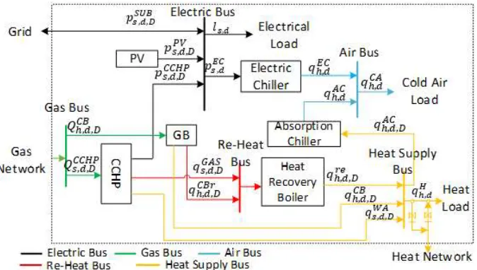
IES usually consist of a CCHP, distributed power sources (adjustable and/or non-adjustable), the electrical load, heating load, cooling load, thermal network, and the electrical network. It can also be connected to the external power grid by a transformer substation. Ref. [29] describes the Busbar structure for IES is shown in Figure 1.
Figure 1. The Busbar structure for integrated energy systems (IES).
In IES, the demands of electricity, heating, and cooling loads can be satisfied simultaneously. The electricity demand is generated by the CCHP, distributed power resources (photovoltaic (PV) cells, for example), and an external grid (when the load demand exceeds the total electricity capacity), and so on. The heating demands are fulfilled by CCHP and the gas boiler, and the cooling demands are met by both an electric chiller and an absorption chiller. The heat recovery boiler (HRB) acts as a waste heat recovery facility, and can collect the waste heat generated by both the CCHP and the gas boiler, which can significantly improve the amount of heat used of the system. The power grid, the thermal equipment linking to the link energy production equipment, and the different loads operate together to achieve energy circulation through the whole system. It is necessary to emphasize that the interaction between the CCHP and the thermal network is bidirectional, so there is a switch apparatus between them to achieve directional selectivity. The heat networks of different regions can also transfer heat through a switch apparatus between the heat exchanger and the heat load.
in these regions, the IEMG can provide a more economical, efficient, and reliable supply of energy for different kind of loads. Furthermore, it can connect to the external power grid and the thermal network, and can thus purchase electricity and heat energy when the overall output in the region is insufficient, or sell surplus energy to external buyers. It can therefore significantly improve the economic efficiency for integrated energy suppliers. To summarize, due to the multi-region and multi-energy complementation, the electricity reliability, economical efficiency, and the comprehensive utilization rate of energy within the region of the IEMG is effectively improved.
Area A CCHP
↓↓↓
Users
Area B CCHP
↓↓↓
Users
Area C CCHP
↓↓↓
Users
Area D CCHP
↓↓↓
Users Area n
CCHP
↓↓↓
Users
Energy Network Topology
Electricity Bus Gas Bus Air Bus Heat Supply Bus
Figure 2. Diagram of the integrated energy micro-grid (IEMG). 2.2. The Principle Elements of the IEMG
The IEMG model in this paper includes three main parts: energy generation, the transformation network, and loads. Generation refers to the electricity, heat, and other energy supply equipment, including the gas combustion engine, CCHP, photovoltaics, substation, and boiler. The network denotes the electrical power grid and the thermal network. The loads are the electrical, heating, and cooling loads. This section models these devices mathematically.
2.2.1. The Generation Equipment (1) CCHP
In this paper, the CCHP is built using a constant efficiency model, and the relationship between its thermoelectric power and fuel consumption is established through approximation of a linear function [30,31].
The fuel combustion of CCHP can be calculated by the following:
𝑄, , = 𝑉, , 𝜃 /3.6
Accordingly, its electrical output is:
𝑝, , = 𝛼 , 𝑄, , + 𝛽,
The net calorific value of the waste heat is:
𝑞, , = 𝛼 , 𝑄, , + 𝛽 ,
The net calorific value of the jacket-cooling water is:
𝑞, , = 𝛼 , 𝑄, , + 𝛽 ,
The expression of fuel combustion describes the total calorific value 𝑄, , converted from the
combustion inflow 𝑉, , (unit: m³/h) per unit time, where 𝜃 is the average calorific value (which
and the available calorific value in the waste heat generated by CCHP. In these equations, 𝑝, , is
the power output of CCHP; 𝑞, , and 𝑞, , are the net calorific values of the waste heat and the
jacket-cooling water, respectively, in kW. The parameters 𝛼 and 𝛽 are two known coefficients that
are used to fit the performance of the CCHP. In practice, the output of the CCHP is subject to other technical constraints, including the service life of the unit, the maximum and minimum output limitation, the ramp rate of the unit, the minimum continuous running time, and the minimum continuous downtime. These constraints and parameters are selected differently during the different optimizing purposes. The main purpose of this paper is the planning and optimization of IEMG. Therefore, the specific constraints and parameter selection will be detailed later.
(2) Distributed Generation
The distributed generation in this paper is the PV power generation system, and the mathematical model applied is as follows. The output of a PV system is affected by weather,
temperature, and solar illumination. If the PV output is 𝑝, , , it can be modeled as:
𝑝, , = 𝜁 𝜁,
𝐴 ∙ 𝑓 𝜂[1 + 𝛼 (𝑇 − 𝑇 )]
where 𝜁 is the actual illumination intensity during the tth hour (kW); 𝜁
, is the illumination
intensity under standard conditions; A is the total area of the PV panels, which is: 𝐴 = ∑ 𝐴 , in
which, 𝐴 is the area of a single panel; 𝑓 is the power derating factor of the PV system, denoting
the ratio of the actual output power to the rated output power, which is used to represent the power loss caused by dirt, rainwater, or snow on the PV panels, and by the aging of the panels (its value
here is taken to be 0.9); 𝜂 is the overall conversion efficiency of the PV panels: 𝜂 = ∑ 𝐴 𝜂 , in
which 𝜂 is the conversion efficiency of a single panel (kW); 𝛼 is the power temperature coefficient
(%/℃) (which is generally −0.47); 𝑇 is the reference temperature of the PV generation system
measured under standard conditions (25 ℃ here); 𝑇 can be calculated by:
𝑇 = 𝑇 + 0.0138(1 + 0.031𝑇 )(1 − 0.042𝑣 ) ∙ 𝐴
where 𝑇 is the ambient temperature (𝑇 ) and 𝑣 is the wind velocity (m/s).
After building the model of the PV system, it is necessary to describe the relationship between solar radiation and the output of the PV system. The beta-distribution probability function can be used to express the output variation of the PV generation system. According to Ref. [32]:
f(𝑃 ) = 𝛤(𝛼 + 𝛽) 𝛤(𝛼)𝛤(𝛽)
𝑃
𝑅 1 − 𝑃 𝑅
where 𝛼 and 𝛽 are the shape parameters of the beta-distribution; 𝑃 is the total power of the PV
array, and 𝑅 is the maximum power that the PV array can output.
(3) Gas Boiler
The heat required in the IEMG is mainly produced by two devices, a CCHP and a gas boiler. During production, the thermal energy is mainly provided by the CCHP. Once it cannot meet the heating load, the gas boiler (GB) can convert the chemical energy of the fuel into thermal energy with a high conversion efficiency, to achieve the thermal balance of the system. Assuming that the gas boiler converts the energy of the natural gas into heat at a constant conversion efficiency, the thermal power of the natural gas that consumed by the gas boiler is:
𝑄 , , = 𝑉, , 𝜃 /3.6
and the heat supply efficiency is:
𝑞 , , = 𝜂 , 𝑄 , ,
where 𝑄 , , is the thermal power of the fuel consumed by the boiler (kW); 𝑞, , is the boiler’s heat
Similar to the CCHP, some waste heat of the gas boiler can be reused. The formula for the available waste heat efficiency is:
𝑞, , = 𝜂 , 𝑄 , ,
where 𝑞, , is the total available waste heat of the boiler, and 𝜂 , is the waste heat energy
efficiency coefficient of the boiler. (4) Heat Recovery Boiler
The recycling of waste heat is an important means for improving energy efficiency. In IES and IEMGs, a heat recovery boiler (HRB) is used to collect waste heat from the system. The model of the heat recovery boiler is:
𝑞 , = 𝜂 (𝑞, , + 𝑞 , , )
where 𝑞 , is the output of the heat recovery boiler (kW), 𝑞, , is the waste heat from CCHP (kW);
𝑞 , , is the waste heat from gas boiler (kW); 𝜂 is the thermal efficiency of the equipment.
(5) Chiller
There are two kinds of chillers commonly used in IES and IEMGs. These are the absorption chiller (AC) and the electric chiller (EC). ACs are driven by a thermal medium, such as lithium bromide or ammonia solution; during operation, the working medium vaporization absorbs a lot of heat from the refrigerant water, so as to achieve cooling. The refrigeration principle of the EC involves first compressing the gas refrigerant by electricity, then discharging the refrigerant into a condenser. Under set pressure and temperature conditions, the low temperature and low pressure refrigerant cools the air or the condensed water in the condenser to achieve a cooling effect.
The models of the two chillers are as follows. For an AC:
𝑞 , = 𝑞 , ,, ∙ 𝜂 ,
where 𝑞, is the cooling output (kW); 𝑞 , ,, is the heat input (kW); and 𝜂 , is the refrigeration
coefficient, which is the ratio of the heat input to the cooling output, and it is usually used to measure the performance of an AC. For an EC:
𝑞, = 𝑝 , , ,
∙ 𝜂 , ,
where 𝑞, is the cooling output (kW); 𝑝 , ,
, is the electric power input (kW); and
𝜂 , , is the
refrigeration coefficient of the EC.
2.2.2. Energy Network Model
The mathematical expression for the energy network, which connects different devices and different regions in the IEMG, can be represented by network topology. Its connection mode is described by the incidence matrix of the topology structure. It consists of the combination of several IES, as shown in Figure 1, with the framework of Figure 2 as an example. As in Figure 1, suppose that the equipment and energy network connection (both from the power grid and the thermal network) in IEMG are nodes. Each pipe or power line serves as a branch, taking the flow direction of the working medium as the branch direction. A basic model of the energy network expressed by the incidence matrix is by the following. Assume that V is the node set of the network. and E is the set of the power lines or pipes (referred to in the following as the set of edges). The energy network can be
represented by the v by e incidence matrix 𝐴 = [𝐴 ]. Thus, each node of the network is a row of the
incidence matrix, and each edge is a column [33]. The relationship between the nodes and edges can
be indicated by the sign of 𝐴 . When 𝐴 = 1, the node 𝑣 is linked with edge 𝑒 and the direction
points away from 𝑣. When 𝐴 = −1, 𝑣 is also linked with 𝑒 and the direction points towards 𝑣.
When 𝐴 = 0, 𝑣 and 𝑒 are not linked.
accurately, the incidence matrix needs to be further expanded. Based on the form of the incidence matrix A, it is split into the start incidence matrix 𝐴 and the end point incidence matrix 𝐴 , to
represent the node set of the starting or ending points of the power and pipe lines, respectively.
Therefore, 𝐴 and 𝐴 are defined as follows:
𝐴 = (𝑎 ) × ∈ {0,1} ×
𝑎 = 1, (𝑧, 𝑐) = 𝐸 0, else
and
𝐴 = (𝑎 ) × ∈ {0, −1} ×
𝑎 = −1, (𝑐, 𝑧) = 𝐸 0, else
Hence, suppose that the basic loop set of 𝐺(𝑉, 𝐸) is L containing p elements, and its basic loop
matrix is 𝐵 = [𝐵 ]. Thus, in the matrix B, each element 𝐵 describes the relationship of the loop
𝐿 (𝐿 ∈ 𝐿, ℎ = 1,2, … , 𝑝) with edge k (a branch of the grid or pipeline in the thermal network). When
𝐵 = 1, the loop 𝐿 is in the same direction as edge k; when 𝐵 = −1, the loop 𝐿 is opposite to
the edge k. If 𝐵 = 0, the edge k is not in the loop 𝐿 . This method can be used to describe most of
the network system. Ref. [34] summarizes the energy network based on the incidence matrix, and the matrix can express the energy network as:
𝐴𝐻 = 0 𝐵∆𝑋 = 0
where A is the incidence matrix of the energy network, B is the basic loop matrix, H is the energy
extensive flow matrix, and ∆𝑋 is the energy-intensive difference matrix. The equivalent transfer
characteristics for incompressible fluids in the energy network is:
𝐻 = 𝐻∗=𝑋 − 𝑋 𝑅 ,
𝑅 = 𝐿 𝐾𝑆
where H is the flow of energy transferred in the network, 𝐻∗ is the equivalent extensive energy flow
in the transfer process, R is the transmission resistance, L and S are the length and cross-sectional area
of the transmission line, and K is the transfer coefficient of extensibility.
By combining these two equations, the energy transfer characteristic equation set for the energy network can be established in order to describe the energy transfer state at each node. The advantage of the incidence matrix is that it turns the topology relationship, and the structure of the nodes and edges in the network into variables in a matrix, which is convenient for calculations. It is also helpful for making real-time variations of the connection mode during network analysis, and therefore, it simplifies and expands the analysis of the energy network system. In addition, the incidence matrix can be used to calculate the power flow at any position of the energy network, which can improve the accuracy of energy network planning and operation optimization. On the basis of the incidence matrix expression for the energy network, models of the electrical network and the thermal network, and their constraints can be determined, as follows.
(1) Electrical Network Model
Based on the above, by taking into account Kirchhoff’s current law (KCL), Kirchhoff’s voltage law (KVL), and electricity flow constraints for network systems, the power grid model of the IEMG containing the distributed generation sources can be derived.
a. The Kirchhoff’s current constraint (KCL):
This equation reflects the equilibrium relationship between the inlet current and the outlet current at
any node in scenario t. In the equation, 𝑆 is the node-branch incidence matrix of the power grid in
scenario t, 𝑓 is the branch current, 𝐺 is the input power of the node from the power generation
equipment, 𝑟 is the lost electrical load, and 𝑑 is the electrical load at the node.
b. Kirchhoff’s voltage constraint (KVL) and the voltage magnitude constraint are:
𝑍, 𝑓, + [𝑆 ] 𝑉, = 0
𝑉 ≤ 𝑉 ≤ 𝑉
Here, row j is the j-th column, T refers to the transpose, V is the column vector of the node voltage,
and Z is the line impedance. The inequality defines the magnitudes of the node voltage in which 𝑉
and 𝑉 are the maximum and the minimum voltage magnitudes, respectively.
(2) Thermal Network Model
Similar to the above, using the energy network incidence matrix and Kirchhoff’s laws, a model describing the working principles of the thermal network can be established. Three functions are used to define the transmission flow of the working medium, the relationship of heat and flow, and the change of the transmission pressure. In addition, apart from the relationship between the heat transfer and the mass flow, it is necessary to consider the corresponding heat loss [35]. The thermal network model is as follows.
a. The transmission flow constraint:
𝑆 𝑞 + 𝐺 = 𝑑
where 𝑆 is the node–branch incidence matrix of the thermal network in scenario t, 𝑞 is the
energy flow in the branch pipe line in scenario t, 𝐺 is the input power of the node from heat
generation equipment, and 𝑑 is the thermal load at the node.
b. The heat-flow constraint:
According to the equivalent energy transfer characteristic equation for thermal network, the relationship between the available heat and the flow is:
𝑞 = 𝑃 𝑘(𝑇 − 𝑇 )
where 𝑃 is the energy (heat) intensity in the pipeline section, k is the specific heat capacity of the
working medium, 𝑇 and 𝑇 are the feed-water temperature and return-water temperature at the
node, respectively.
c. The transmission pressure constraint:
After the relationship between the heat and the flow in the thermal network has been determined, the heat intensity at the node conforms to the following heat balance constraint:
𝑍, 𝑞, + [𝑆 ] 𝑃, = 0
where 𝑍, is the demand for the thermal intensity at node j during period t; 𝑞, is the energy flow
at node j; 𝑃, is the heat column vector in the pipeline section connected to node j.
2.3. Energy Balance of the IEMG
From the configuration and structure of the IEMG, as shown in Figure 3, the electrical/cooling/heating loads should be balanced in any district, or balanced over the whole region, and in all of the different scenarios this principle is basically the same. The energy balance equations in the IEMG are introduced below.
a. Balance of the electrical load (in all scenarios):
The electrical load balance shall be satisfied in any scenario s (s = c, h, t, e). 𝑝 is the power from
the external grid, 𝑝, is the PV generation power, 𝑝, is the power of the CCHP (kW), 𝑙 , is the
pure electrical load, and 𝑝, is the power of the electric chiller (kW).
b. Balance of the cooling load (in scenarios of a cooling supply period)
The demand for cooling is satisfied by two devices: the electric chiller and the heat adsorption chiller:
𝑞, = 𝑞 , + 𝑞 ,
where 𝑞 , is the total load of cooling, 𝑞 , is the input power of the electric chiller, and 𝑞, is the
input power of the adsorption chiller.
c. The balance of heating load (in the scenario of a heating supply period): The heating load is satisfied by the CCHP and the gas boiler:
𝑞 , = 𝑞 , + 𝑞 ,
where 𝑞 , is the total heating load, 𝑞 , is the heat supplied by the CCHP, and 𝑞, is the heat
from the gas boiler.
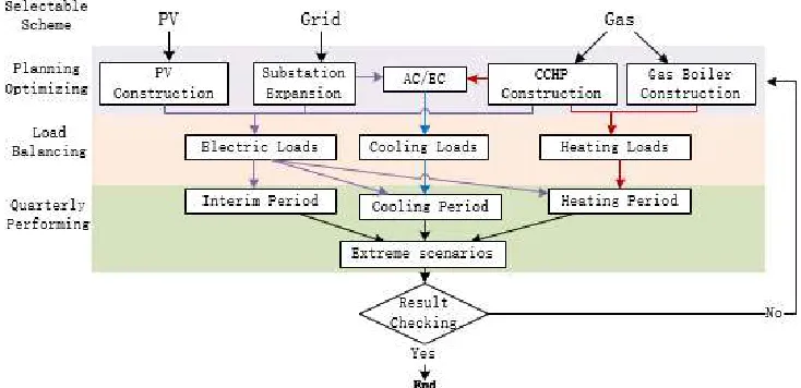
Figure 3. Planning optimization processes of the IEMG. 3. The IEMG Planning Optimization Model
3.1. Planning Process and Framework
In this study, the procedure for IEMG planning is summarized as follows:
(1) Extract the regional division, loads, and other planning-related data and information, and carry
out the overall regional energy supply equipment configuration (for electricity, heating, and cooling).
(2) Obtain the overall configuration capacity of the energy supply equipment from step 1, combined
with the load characteristics of each region, and doing the regional equipment type selection and capacity optimization.
(3) According to the equipment selection and capacity optimizing results, deduce the electricity,
heating and the cooling load balance operation simulation of each region, and output the results.
(4) Deduce the load balance operation simulation on the basis of quarterly and extreme scenarios,
and output the results.
(5) Test and determine whether the regional and quarterly simulation results conform to the energy
flow and all other constraints.
(6) If the result does not satisfy all the constraints, adjust the selection and capacity results until all
In the steps above, Step (1) is preparatory work. Its main function is to determine the macroscopic capacity of the whole region on the basis of the known information, in order to narrow the scope of subsequent optimization. Step (2) determines the equipment selection and the installed capacity of each region on the basis of the macro-planning results. Steps (3) and (4) formulate the operation strategy and calculate the system operation cost. This is done through regional and situational operation simulation, using the planning scheme and the scenarios determined in the previous steps. Steps (5) and (6) ensure that the results meet the requirements of the constraints, and improve the accuracy of the optimization. The process is also shown in Figure 3.
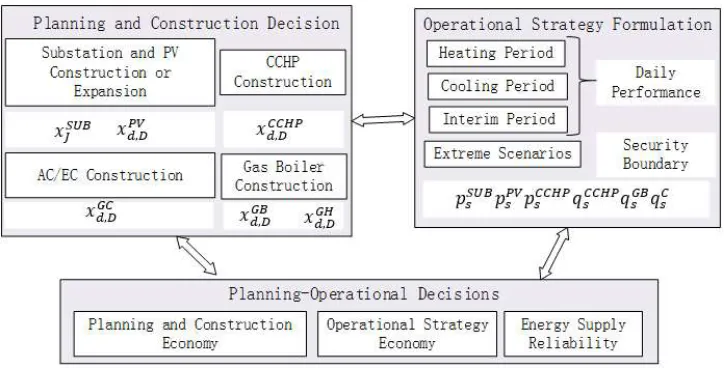
Assume that an IEMG satisfies its electrical/heating/cooling loads through PV panels, natural gas (for the CCHP and gas boiler), as well as by purchasing electricity from the external grid. It is then necessary to consider the IEMG plan from the aspect of expanding its original capacity or building a new transformer substation and PV system to supply electricity. A new CCHP construction can meet the electrical/cooling/heating energy demands. Increasing the number of gas boilers compensates for heating between the CCHP heating output and the heating demand. Adding more chilling equipment can satisfy the cooling load. Accordingly, the decision process of the IEMG planning model is given as in Figure 4.
Figure 4. The main variables and decisions of the IEMG planning model.
Thus, the decision variables in the model can be classified into two types: construction and operation.
The constructional decision variables are mainly binary, where ‘0’ and ‘1’ mean to undo/do
decision, respectively. To be specific, in the type selection option d, 𝑥 , is the decision variable for
whether to invest in the new CCHP in district D or not; similarly, 𝑥 , is the decision variable of any
other power generator in district D. 𝑥 , is the decision variable of the heating generator, 𝑥 , is the
decision variable of the cooling generator, and 𝑥 is the decision variable of a new or expanded
transformer substation.
The operation decision variables are continuous and include: the electrical generation output of
the CCHP, 𝑔 ; the heating generation output of the CCHP, 𝑞 ; the heating power of the gas
boiler, 𝑞 ; the power of the electricity purchased from the external gird to the substation, 𝑔 ; and
the power of the cooling generation equipment, 𝑞 .
3.2. The Objective Function
The overall objective of the planning model is to meet the maximum energy needs of the whole region while minimizing the sum of the construction cost and the operation cost. Hence, the objective function in this model consists of three parts: the planned construction cost, the planned operation cost, and the value of lost loads:
min 𝐶 + 𝐶 + 𝐶
where 𝐶 is the planned construction cost, 𝐶 is the planned operation cost, and 𝐶 is the
value of lost load. The calculation of each part is as follows. (1) The planned construction cost:
The function of the planning model is to select the economic optimal among several construction schemes, then it should be noticed that there are many different supplement construction portfolios, the equation below gives the cost which is determined to be constructed. Now, assume that plan D
is known to be executed, thus, the planned construction cost 𝐶 of plan D includes the construction
cost of the CCHP, the construction cost of the electrical/cooling/heating generator, and the expansion cost of the transformer substation:
𝐶 = 𝑀 , 𝑥 , ∈ф
∈Ω
+ 𝑀 𝑥
∈ф
+ 𝑀 , 𝑥 , ∈ф
∈Ω
+ 𝑀, 𝑥 ,
∈ф ∈Ω
+ 𝑀 , 𝑥 ,
∈ф ∈Ω
+ 𝑀 , 𝑥 ,
∈ф ∈Ω
where 𝑀 , , 𝑀 , , 𝑀 , , 𝑀 , , and 𝑀 , are the construction costs of PV panels, the CCHP, the gas
boiler, the heating equipment, and the cooling equipment, respectively, in region d. 𝑀 is the cost
of expanding the transformer substation (J represents plan J); and x is a binary decision variable,
where the cost is taken into account when the value is 1. (2) The planned operation cost:
Here, equipment maintenance and depreciation costs are put aside. The planned operation cost
𝐶 includes the cost of the fuel for the CCHP and the gas boiler, and the cost of purchased
electricity:
𝐶 = 𝑟
(1 + 𝑖) 𝜀 (𝑃𝑟 𝐹, + 𝑃𝑟 𝑝, ) , ,
∈Ω
where r represents the system run cycle, ∑
( ) is the total net cost of the annual operation, i is the
discount rate, and 𝜀 is the proportional contribution of scenario s to the entire planning period. For
instance, when the planning period is one year (12 months), if the heating supply period contains four months from 15 November to 15 March, the proportion is 4/12 = 0.333; if the cooling supply period contains three months from 15 June to 15 September, the proportion is 3/12 = 0.25, then the
transitional period contains the other five months and the proportion is 5/12 = 0.417. 𝑃𝑟 and
𝑃𝑟 are the prices of natural gas and external electricity, respectively. 𝐹, is the fuel
consumption per unit time in district d, which consists of the fuel consumed by the CCHP and the
gas boiler:
𝐹, = ∑ ∈ф 𝐹, , + ∑ ∈ф 𝐹, , .
𝑔, is the quantity of the electricity purchased from the external grid by a substation in district d.
(3) The value of the lost load:
In this part, 𝐶 indicates the compensation cost for unsatisfied electrical/heating/cooling
loads, which are not supplied during scenario s in district d.
𝐶 = 𝑃 𝑅 , , ∈Ω
Here, 𝑅 , is the capacity of the lost loads and 𝑃 is the cost coefficient of the lost loads. It should
be pointed out that 𝑃 is set to a relatively high value, in order to avoid load loss during
operation.
3.3. Constraint Conditions
In planning the IEMG, the variation of generation equipment parameters in the model should be within a certain range. Their constraint conditions are given in the following.
a. The permeability constraint on the distributed generation (DG)
The proportion of the DG to the total installed capacity should be within a certain range:
𝑝 ,, ≤ 𝑝 , ≤ 𝑝 , ,
𝑣 ,, ≤ 𝑣 , ≤ 𝑣 , ,
𝑁, , ≤ NG , ≤ 𝑁, ,
where in the plan D for region d, 𝑝 , , and 𝑝 ,, are the lower and upper limits of the active
power of the DG (kW). 𝑣 ,, and 𝑣 ,, are the lower and upper limits of the reactive power
(kW) of DG, respectively. 𝑝 , and 𝑣 , are the actual active power and reactive power of DG in
district d (kW). 𝑁 , , and 𝑁 , , are the lower and upper limits of the number of the DG in the
system. NG , is the number of DGs in district d.
b. Operational constraints for the CCHP:
The operational constraints for the CCHP include the maximum and the minimum outputs, the ramp rate, and the maximum and the minimum continuous running times. They are given by:
𝑥 , ∈ф
𝑝 , , ≤ 𝑝 , ≤ 𝑥 , ∈ф
𝑝 , ,
where 𝑝 , , and 𝑝 , , are the lower and the upper limits of the CCHP’s output (kW).
The number of generation units in each district needs to be limited, due to geographical factors. In this model, we only limit the total number of CCHP units, and allow one per district:
𝑋 , ∈ф
≤ 1
where 𝑋 , is the total number of CCHP generation units in district d. This constraint can be
adjusted according to planning requirements. c. Operation constraints on the gas boiler:
The output heating power of the gas boiler during operation should be no larger than its rated power:
0 ≤ 𝑞 , ≤ 𝑥 , 𝑞 , , ∈ф
where 𝑞 , , is the rated power.
Similarly, the construction constraint for the gas boiler is:
∑ ∈ф 𝑋 , ≤ 1.
This ensures that the boilers in district d are of the same capacity.
d. Constraints on the chillers:
The power of the adsorption chiller and the electrical chiller during operation should be no larger than their rated power:
0 ≤ 𝑞, / ≤ 𝑞 /, ,
where 𝑞 /, , is the rated power of the chiller (kW).
The power flow of the system should be limited according to the magnitude of the current in the electrical network:
|𝑓 | ≤ 𝑦 𝑓
where 𝑓 is the upper limit of the current magnitude and 𝑦 is the conductance value at the
corresponding node.
g. The balance constraint for heat loss in the thermal network:
If there is too much heat loss in the pipelines of the thermal network, the temperature of the working medium in the pipelines will become lower than the temperature of the working medium in the return-water system. As a result, the thermal network will be ineffective. To ensure the efficiency of the thermal network, we therefore need to ensure that the power (temperature) of the usable heat in the pipelines is higher than a critical value and lower than the maximum power that can be transferred in the pipelines:
𝑃 ≤ 𝑃,∗≤ 𝑃
where 𝑃,∗ is the power of the usable heat in the working medium at node j, 𝑃 is the lower critical
value of the power of the usable heat, and 𝑃 is the maximum power of the usable heat. If the
working medium flows away from node i then the value of 𝑃,∗ is positive, otherwise it is negative.
h. The supply capacity constraint for the transformer substation (in the external grid):
In the transformer substation, the total power supply capacity should not be greater than the product of the load and the capacity–load ratio, expressed as:
𝛾 𝑝 ≤ 𝑝 + 𝑥 𝑝 ∅
≤ 𝛾 𝑝
𝑥 ∅
≤ 1
The first inequality describes the relationship between the original power supply capacity 𝑝 and
the expanded capacity ∑ ∅ 𝑥 𝑝 . The sum is the expanded total power supply capacity. To
ensure accuracy and effectiveness in planning, the product of the total power supply capacity and
capacity–load ratio 𝛾 should be valid for the extreme load scenario (s=e). The range of the capacity–
load ratio 𝛾 in this model is 1.8~2.1. The second inequality means that only one transformer
substation expansion plan in the set ∅ will be carried out.
3.4. Calculation Method
We used the mixed integer linear programming (MILP) method to solve the IEMG planning model. The model involves the following decision variables: the output of the PV power system, the input and outputs of the CCHP, the electricity purchased from or sold to the external power grid, the input of the conversion equipment, and the input and output of the gas boiler. The model can be solved using a mature algorithm, or directly by commercial software, such as CPLEX, GUROBI, and LINGO [36]. In this study, the model was built by the software MatLab and yalmip, and solved by the optimization software GUROBI.
4. Case Study
4.1. Case Description
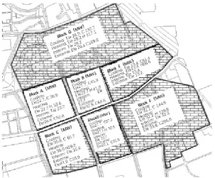
Figure 5. Map showing the energy supply planning information of the case study area.
From Figure 5, the data of the loads were classified under four scenarios: cooling period, heating period, transitional period, and extreme cooling period. It should be noted that during the calculation the load on the air conditioner should be subtracted during the cooling period.
Alternative planning options for the energy supply in the region are listed in Table 1. The parameters of the different CCHP units are listed in Table 2. The parameters used for the 9.5 MW CCHP unit are the same as those for the 5 MW unit.
Table 1. Alternative planning options for the energy supply equipment. CCHP, PV, AC, EC, HRB; CNY: Chinese CNY.
Substation Expansion CCHP
Scheme
No. Capacity (MVA) Construction Cost Scheme No. Capacity (MW) Construction Cost
1 1 × 50 800 1 1 1200
2 2 × 50 1600 2 2 2400
3 3 × 50 2400 3 3 3500
4 4 × 50 3200 4 5 5400
5 5 × 50 4000 5 9.5 10,260
6 6 × 50 4800
Gas Boiler Others
Scheme
No. Options (MW) Alternative Construction Cost Equipment Construction Cost Unit
1 50 2857 PV 850 10 CNY/MW
2 100 5714 AC 60 10 CNY/MW
3 150 8571 EC 85 10 CNY/MW
4 200 11,430 HRB 15 10 CNY/MW
(unit: 10 CNY)
Table 2. Performance Parameter of CCHP. Full Capacity
(MW) 𝜶𝑮𝑬 Characteristic Function Coefficient 𝜷𝑮𝑬 𝜶𝑮𝑨𝑺 𝜷𝑮𝑬 𝜶𝑾𝑨 𝜷𝑾𝑨
2 0.466 −657.422 0.219 13.644 0.151 90.737
3 0.479 −758.940 0.208 94.383 0.153 173.562
5 0.472 −896.264 0.207 125.832 0.149 204.828
9.5 0.470 −915.262 0.204 130.261 0.146 220.152
Other operation parameters included the calorific value and price of gas: 32.967 MJ/m3 and 3.23
CNY/m3, respectively (CNY is Chinese CNY); the external electricity price in this area was a
commercial price, which was 0.9923 CNY/kWh (the purchase price from the weighted average of the
peak–valley electricity prices). The total planning period was 10 years and the annual discount rate i
was 5%. To minimize the lost load, the value of 𝑃 was set to be 1,000,000 × 104 CNY/MW.
Four cases were set to make the calculation of the planning more accurate:
CASE 1—Electricity is only purchased from the external power grid, without consideration of PV and CCHP;
CASE 2—At least a 4 MW PV system is built in each district and electricity can be purchased from the external power grid, without consideration of the CCHP;
CASE 3—CCHP construction is considered and electricity can be purchased from the external power grid when the output of the CCHP is insufficient, without consideration for PV;
CASE 4—At least a 4 MW PV generation system is built in each district, CCHP is considered, and electricity can be purchased from the external power grid when the outputs of the CCHP and the PV are insufficient.
4.2. Results and Analysis
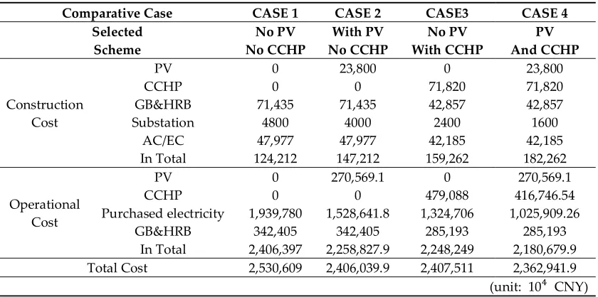
The economic calculation results of the IEMG planning are shown in Table 3.
Table 3. Cost comparison of the different case study scenarios.
Comparative Case CASE 1 CASE 2 CASE3 CASE 4
Selected
Scheme No CCHP No PV No CCHP With PV With CCHP No PV And CCHP PV
Construction Cost
PV 0 23,800 0 23,800
CCHP 0 0 71,820 71,820
GB&HRB 71,435 71,435 42,857 42,857
Substation 4800 4000 2400 1600
AC/EC 47,977 47,977 42,185 42,185
In Total 124,212 147,212 159,262 182,262
Operational Cost
PV 0 270,569.1 0 270,569.1
CCHP 0 0 479,088 416,746.54
Purchased electricity 1,939,780 1,528,641.8 1,324,706 1,025,909.26
GB&HRB 342,405 342,405 285,193 285,193
In Total 2,406,397 2,258,827.9 2,248,249 2,180,679.9
Total Cost 2,530,609 2,406,039.9 2,407,511 2,362,941.9
(unit: 10 CNY)
substation is 2 × 50 MVA, the construction cost is 1.822 billion CNY, and the total planning cost is 21.82941 billion CNY.
In CASE 1, the demands for electricity are satisfied by purchasing electricity from external power grid and heating are from the gas boiler. This scheme involved the least equipment. The system’s structure was relatively simple, and the construction cost was therefore the lowest, but the energy supply form was simple and the operational cost was relative high: 19.397 billion and 3.424 billion CNY for electricity and heat, respectively, and 24.063 billion CNY in total (which is the highest of the four CASES). In CASE 2, due to PV sources in each district (28 MW in total), the construction cost of the whole system was increased by 18.52% compared to CASE 1. However, the operation cost of the external electricity was lower, and the thermal generation’s cost remained unchanged, leading to CASE 2 having a 5.31% reduction in operation cost and a 4.13% decrease in total planning costs. In CASE 3, a CCHP system was added to supply electricity and thermal energy. Compared to CASE 1, the construction cost was 28.22% higher, but due to the application of the CCHP the cost of purchasing electricity was 31.71% lower. The cost of the heating supply was 16.70% lower, and thus the total cost decreased by 4.86%. In CASE 4, both PV and CCHP are constructed, which meant that the scheme combines the characteristics of cases 2 and 3. Therefore, compared to CASE 1, the construction cost was 46.73%, higher but the operation cost decreased by 9.37%. Lower operating costs offset the higher construction costs, making CASE 4 the lowest costing among the four cases. Therefore, in CASES 2, 3, and 4, the total planning–operation costs were decreased by 3.74%, 4.86%, and 6.63% compared to CASE 1, respectively. To sum up, the application of PV and the CCHP in the IEMG is efficient in reducing the total planning–operation cost as a whole.
5. Conclusions
This paper presents an IEMG planning model which balances electrical/cooling/heating loads in multiple districts. In this model, district energy suppliers are seen as the main investors, who are responsible for supplying cooling/heating/electrical power in the districts, and the costs they invest in construction and operation were investigated. Optional energy supply plans include: building a new PV generator, expanding existing transformer substations, building a CCHP, and increasing the number of gas boilers and electric chillers, and so on. The operation is analyzed on the basis of different scenarios: heating period, cooling period, and transitional period; extreme situations are also taken into consideration, to make sure that the system is reliable. A development zone including seven districts, was taken as a case study to test the validity of the model, and four cases were considered: CASE 1 (electricity supplied by an external power grid), CASE 2 (electricity supplied by an external power grid and PV), CASE 3 (electricity supplied by an external power grid and a CCHP), and CASE 4 (electricity supplied by an external power grid, PV, and a CCHP). The calculations show that during the 10 years of the planning period, the order of the construction costs is CASE 4 > CASE 3 > CASE 2 > CASE 1; however, because the planning period is long and the operation costs are much higher than the construction cost, the order of the total costs is CASE 1 > CASE 2 > CASE 3 > CASE 4. Compared to CASE 1, the total planning–operation costs in the other three cases are decreased by 3.74%, 4.86%, and 6.63%, respectively, which reflects that the construction of the distributed PV and CCHP generation sources are beneficial for reducing the total planning–operation costs.
discussed, without consideration of the variation of energy quantity flow rate, the variations of temperature and pressure in the thermal network, and time delays in the thermal network’s heat transmission. In addition, the planning and construction of the framework of the energy network was not fully investigated. Thus, the study could be further improved in the future by considering these aspects.
Author Contributions: Methodology, H.H., and Z.T.; Writing-Original Draft Preparation, H.H.; Writing-Review & Editing, all the authors.
Funding: This research was funded by National Natural Science Foundation of China under Grant No.71774039. Conflicts of Interest: The authors declare no conflict of interest.
References
1. Sun, H.; Guo, Q.; Pan, Z. Energy Internet: Concept, Architecture and Frontier Outlook. Autom. Electr. Power Syst. 2015, 39, 1–3, doi:10.7500/AEPS20150701007.
2. Yao, J.; Gao, Z.; Yang, S. Understanding and Prospects of Energy Internet. Autom. Electr. Power Syst. 2015, 39, 9–14, doi:10.7500/AEPS20151101004.
3. Jia, H.; Wang, D.; Xu, X.; Yu, X. Research on Some Key Problems Related to Integrated Energy System. Autom. Electr. Power Syst. 2015, 39, 198–207, doi:10.7500/AEPS20141009011.
4. Dong, C.; Zhao, J.; Wen, F.; Xue, Y. From Smart Grid to Energy Internet: Basic Concept and Research Framework. Autom. Electr. Power Syst. 2014, 38, 1–7, doi:10.7500/AEPS20140613007.
5. Mancarella, P. Distributed multi-generation options to increase environmental efficiency in smart cities. In Proceedings of the 2012 IEEE Power and Energy Society General Meeting, San Diego, CA, USA, 22–26 July 2012.
6. Chicco, G.; Mancarella, P. Distributed multi-generation: A comprehensive view. Renew. Sustain. Energy Rev. 2009, 13, 535–551.
7. Gu, W.; Wu, Z.; Bo, R.; Liu, W.; Zhou, G.; Chen, W.; Wu, Z. Modeling, Planning and Optimal Energy Management of Combined Cooling, Heating and Power Microgrid: A Review. Int. J. Electr. Power Energy Syst. 2014, 54, 26–37.
8. Wang, R.; Gu, W.; Wu, Z. Economic and Optimal Operation of Combined Heat and Power Microgrid with Renewable Energy Resources. Autom. Electr. Power Syst. 2011, 35, 1–6.
9. Liu, X.; Wu, H. A Control Strategy Operation Optimization of Combine Cooling Heating and Power System Considering Solar Comprehensive Utilization. Autom. Electr. Power Syst. 2015, 39, 1–6, doi:10.7500/AEPS20140626004.
10. Gu, W.; Wu, Z.; Wang, R. Multi-Objective Optimization of Combined Heat and Power Microgrid Considering Pollutant Emission. Autom. Electr. Power Syst. 2012, 36, 1–9.
11. Guo, L.; Liu, W.; Cai, J.; Hong, B.; Wang, C. A Two-stage Optimal Planning and Design Method for Combined Cooling Heating and Power Microgrid System. Energy Convers. Manag. 2013, 74, 433–445. 12. Wu, Q.H.; Zheng, J.H.; Jing, Z.X. Coordinated Scheduling of Energy Resources for Distributed DHCs in an
Integrated Energy Grid. CSEE J. Power Energy Syst. 2015, 1, 95–104.
13. Wang, J.; Li, X.; Yang, H.; Chen, G. An Integration scheme for DES/CCHP Coordinated with Power System. Autom. Electr. Power Syst. 2014, 38, 16–21, doi:10.7500/AEPS20130523006.
14. Xu, X.; Jia, H.; Jin, X.; Yu, X.; Mu, F. Study in Hybrid Heat-gas-power Flow Algorithm for Integrated Community Energy System. Proc. CSEE 2015, 35, 3634–3642.
15. Khalesi, N.; Rezaei, N.; Haghifam, M.R. DG allocation with application of dynamic programming for loss reduction and reliability improvement. Int. J. Electr. Power Energy Syst. 2011, 33, 288–295.
16. Carpaneto, E.; Chicco, G.; Mancarella, P.; Russo, A. Cogeneration planning under uncertainty. Part I: Multiple time frame approach. Appl. Energy 2011, 88, 1059–1067.
17. Carpaneto, E.; Chicco, G.; Mancarella, P.; Russo, A. Cogeneration planning under uncertainty. Part II: Decision theory-based assessment of planning alternatives. Appl. Energy 2011, 88, 1075–1083.
19. Zhou, R.; Ran, X.; Mao, F.; Fu, J.; Li, X.; Lin, L. Energy-Saving Coordinated Optimal Dispatch of Distribute Combined Cool, Heat and Power Supply. Power Syst. Technol. 2012, 6, 8–14.
20. Wang, C.; Hong, B.; Guo, L.; Zhang, D.; Liu, W. A General Modelling for Optimal Dispatch of Combined Cooling, Heating and Power Microgrid. Proc. CSEE 2013, 31, 26–34. (In Chinese)
21. Kellogg, W.D.; Nehrir, M.H.; Venkataramanan, G.; Gerez, V. Generation unit sizing and cost analysis for stand-alone wind, Photovoltaic, and Hybrid Wind/PV System. IEEE Trans. Energy Convers. 1998, 13, 70–75. 22. Fu, L.; Wang, S.; Zhang, Y.; Zhang, Z.; Dong, P. Optimal Selection and Configuration of Multi-Types of
Distributed Generators in Distribution Network. Power Syst. Technol. 2012, 1, 79–84. (In Chinese)
23. Ge, S.; Yan, C.; Liu, H.; Zhao, B.; Ge, L. Optimal Locating and Sizing of Distributed Generations in Distribution Network. Proc. CSU-EPSA, 2016, 28, 8–15. (In Chinese)
24. Shen, X.; Han, Y.; Zhu, S.; Zheng, J.; Li, Q.; Nong, J. Comprehensive Power-supply Planning for Active Distribution System Considering Cooling, Heating and Power Load Balance. J. Power Syst. Clean Energy 2015, 3, 485–493.
25. Zhang, J.; Yuan, X.D.; Yuan, Y.B. A novel genetic algorithm based on all spanning trees of undirected graph for distribution network reconfiguration. J. Mod. Power Syst. Clean Energy 2014, 2, 143–149, doi:10.1007/s40565-014-0056-0.
26. Wang, C.S.; Chen, K.; Xie, Y.H.; Zheng, H.F. Siting and sizing of distributed generation in distribution network expansion planning. Autom. Electr. Power Syst. 2006, 30, 38–43. (In Chinese)
27. Haffner, S.; Pereira, L.F.A.; Pereira, L.A.; Barreto, L.S. Multistage model for distribution expansion planning with distributed generation—part I: Problem formulation. IEEE Trans. Power Deliv. 2008, 23, 915–923. 28. Fang, C.; Zhang, X.; Cheng, H.; Zhang, S.; Yao, L. Framework planning of distribution network containing
distributed generation considering active management. Power Syst. Technol. 2014, 38, 823–829. (In Chinese) 29. Wang, C,; Hong, B.; Guo, L.; Zhang, D.; Liu, W. A General Modeling Method for Optimal Dispatch of Combined Cooling, Heating and Power Microgrid. J. Proceedings of the CSEE. 2013, 11, 26-35. (In Chinese) 30. Zhang, Q. Siting and Sizing of DG in Distributed Network Planning. Master’s Thesis, Shandong University,
Jinan, China, 2008. (In Chinese)
31. Li, J.X.; Zheng, J.H.; Zhu, S.Z.; Li, Q.S. Economic operation research of CCHP system based on interior point method. East China Electr. Power 2014, 42, 424–430. (In Chinese)
32. Tina, G.; GaGliano, S.; Raitis, S. Hybrid solar/wind power system probabilistic modelling for long-time performance assessment. Sol. Energy 2006, 80, 578–588.
33. Chen, H.; Wen, J.; Wang, Z.; Yang, X. Transfer Laws and Equations of Energy Network. J. Xi’An JiaoTong Univ. 2014, 48, 66–78. (In Chinese)
34. Xie, J.; Xing, W.; Wang, Z. Network Optimization; Tsinghua University Press: Beijing, China, 2000; pp. 3–11. (In Chinese)
35. Wang, G.; Zhang, G. Research of fluid gird method based on power plant thermodynamic system. Mod. Electr. Power 2005, 22, 38–41. (In Chinese)