Compared Computational Performances of EFG Meshfree Metod for One-Dimensional Elastic Problem Analysis

© 2015 IJSRST | Volume 1 | Issue 1 | Print ISSN: 2395-6011 | Online ISSN: 2395-602X Themed Section: Science and Technology

Compared Computational Performances of EFG Meshfree Metod

for One-Dimensional Elastic Problem Analysis

Prof. Sanjaykumar D. Ambaliya

, Prof. Tushar P. Gundaraniya

1

Department of Mechanical Engineering, Government Engineering College, Surat, Gujarat, India

2

Department of Mechanical Engineering, Government Engineering College, Dahod, Gujarat, India

ABSTRACT

Mesh free (MF) methods are among the breed of numerical analysis technique that are being vigorously developed to avoid the drawbacks that traditional methods like Finite Element method (FEM) possess. The Element Free Galerkin (EFG) method is a meshless method in which only a set of nodes and a description of model’s boundary are required to generate the discrete equations. EFG approach is based on global weak form of governing differential equation and employs Moving Least Square (MLS) approximants to construct shape functions. While deriving solution with EFG, following selectable parameters affect solution accuracy and computational efforts: Order of monomial basis function and weight function selection in MLS approximants, size of influence domain, uniform and non uniform node distribution, number of Gauss points in integration cells. The computational performance of meshfree Moving Least Squares technique when solving the Galerkin weak form of one-dimensional elastic problem is tested against exact analytical solution and mesh-based Finite Element Method. In the present paper, selectable parameters are studied to check its influence on solution accuracy in EFG and suggest near optimal selection. Finally, when EFG results are compared with standard FEM solution, it is found that EFG displacements are more accurate than FEM.

Keywords: EFG, MLS Shape Functions, Weight Functions, Meshfree, Matlab, Monomial Basis, Size Of Influence Domain.

I.

INTRODUCTION

The development of the finite element method (FEM) in the 1950s was one of the most important advances in the field of numerical methods. The FEM is a robust and thoroughly developed method, and hence it is widely used in engineering fields due to its versatility for complex geometry and flexibility for many types of linear and non-linear problems. This mesh based numerical methods (FEM, FDM, CFD etc.) despite of great success; suffer from difficulties in some aspects, which limit their applications in many complex problems such as crack propagation, problems with phase change, large-strain deformations, etc. [1]

In recent years, meshless methods have been developed as alternative numerical approaches in efforts to eliminate known drawbacks of the finite element method

method use shape functions which are derived from moving least square (MLS) approximation. In 1981, Lancaster and Salkauskas formulated the Moving Least square approach [Lancaster, 1981]. Nayroles et al (1992) first used it for meshfree approximation and the idea was further formulated into EFGM framework by Belytschko et al (1994). MLS involves the assumption of the field variable as a summation of series of monomials. The coefficients of the monomials are the unknowns and are calculated such that the squared sum of errors in the domain of a point is minimal. Once the approximation at a point is over, the MLS is ‘moved’ to another point. This paper evaluates effect of each selectable significant parameters on EFG solution individually, which includes monomial basis order and weight function selection in MLS approximants, size of influence domain, uniform and non-uniform node distribution, number of Gauss points in integration cells.

II.

METHODS AND MATERIAL

2. EFG FORMULATION:

An axially loaded bar [2] problem is selected for detailed study of selectable parameters in EFG. Considering one dimensional unit length and unit area bar subjected to linear body force which is fixed at one end and free to deform at the other as shown in Figure 1.

Figure 1: Axially loaded bar

Figure 2. Bar with node and integration cell

The bar geometry is defined with eleven uniformly spaced nodes, as shown in figure 2.

u x

( )

p x a x P x a x







Where, PT (x) is monomial basis functions of order m and a(x) are vector coefficients.

The choice of the polynomial function is depends upon the basis and is decided by the Pascal’s triangle. For example, for 1-D problems,

Consider a displacement function u(x) of a field variable defined on the domain Ω, the MLS approximant uˆ(x)of the function u(x) can be represented as,

The unknown parameters a(x) at any given point are determined by minimizing the difference between the local approximation at that point and the nodal parameters ui. Let the nodes whose supports include xbe given local node numbers 1 to n. In order to determine the unknown coefficients a, a functional J is constructed. It sum up the weighted quadratic error for all nodes inside the support domain as

Where n is the number of nodes in the neighbourhood of

x for which the weight function, W(x — xi) ≠ 0, and ui refers to the nodal parameter of u at x = xi.

We want to minimize this functional, so we differentiate with respect to the unknown vector a(x), containing the coefficient,

J

a





=

0

Which results in the following compact matrix form

as,

A x a x

( ) ( )



B x u

( )

1

( )

( ) ( )

a x



A

x B x u

Where,

1 1 1

1

(

) ( )

( )

n

T

I

A

w x

x P x P

x









1 1 2

( )

[ (

) ( ), (

),... (

) (

)

B x



w x



x P x

w x



x

w x



x P x

[

,... ]

By inserting this expression, we get a new formulation of the displacement field,

Where, the shape function is defined by,

1 1

1

( )

( )(

( ) ( ))

n

T

I I I

i

x

P x A

x B x

p A B











A set of discrete system equations is generated on the basis of Galerkin weak form of governing differential equation [2]. Following weak form is used for deriving system equations. Presently, Lagrange multiplier technique is employed for imposing EBCs.

Where, Γu and Γt are essential and natural boundaries respectively [2, 3]. Discrete equations can be obtained by substituting trial (shape) and test (weight) functions in the above weak form. For EFG, test functions are selected as approximating functions, δv = u and final form of linear algebraic equation will be,

0 T

K G u f

G



     _

   

 

     

1

, 0

,

IJ I x J x

K







E



dx

GIK  



1

0

I x t I

f





It







bdx

q

 

u

In which, K is the stiffness matrix, G is the boundary condition matrix, u is the nodal displacements vector, λ

is the Lagrange multipliers, f is the force vector and q is a boundary condition vector, and E is Young's modulus.

3. Weight Functions

The weights functions like cubic weight function, quartic weight, exponential weight etc, perform two actions, one as a medium of imparting smoothness or desired continuity to the approximation and other one, more important, is the establishment of the local nature of the approximation [1]. The weight functions chosen for construction of shape function are as follows:

Where, s= |x-xI|/dmax and, dmax is the size of the support for weight function wi and determines support of node xi. The size of support, dmax, of the weight function wi associated with node i should be chosen such that dmax should be large enough to have sufficient number of nodes covered in the domain of definition of every sample point to ensure the regularity of matrices.

III.

RESULT AND DISCUSSION

The bar problem formulated above, is studied in detail with the help of MATLAB program. The computational performance of EFG method is compared with different significant parameter as discussed below.

4.1 Weight Function and Nodal Distribution:

(A) Regular nodal distribution:

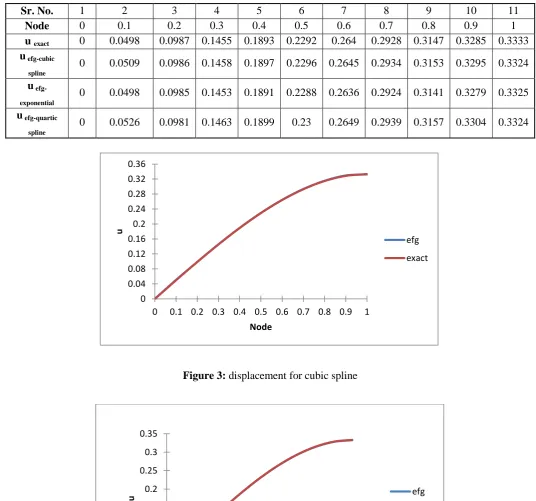
Table 1. Comparison of different weight functions for displacement

Sr. No. 1 2 3 4 5 6 7 8 9 10 11

Node 0 0.1 0.2 0.3 0.4 0.5 0.6 0.7 0.8 0.9 1

u exact 0 0.0498 0.0987 0.1455 0.1893 0.2292 0.264 0.2928 0.3147 0.3285 0.3333

u efg-cubic

spline

0 0.0509 0.0986 0.1458 0.1897 0.2296 0.2645 0.2934 0.3153 0.3295 0.3324

u

efg-exponential

0 0.0498 0.0985 0.1453 0.1891 0.2288 0.2636 0.2924 0.3141 0.3279 0.3325

u efg-quartic

spline

0 0.0526 0.0981 0.1463 0.1899 0.23 0.2649 0.2939 0.3157 0.3304 0.3324

Figure 3: displacement for cubic spline

Figure 4 : displacement for exponential

0 0.04 0.08 0.12 0.16 0.2 0.24 0.28 0.32 0.36

0 0.1 0.2 0.3 0.4 0.5 0.6 0.7 0.8 0.9 1

u

Node

efg

exact

0 0.05 0.1 0.15 0.2 0.25 0.3 0.35

0 0.1 0.2 0.3 0.4 0.5 0.6 0.7 0.8 0.9 1

u

Node

efg

Figure 5 : displacements for quartic spline

(B) Irregular Nodal Distribution

Table 2. Comparison of different weight functions for displacement

Sr. No. 1 2 3 4 5 6 7 8 9 10

Node 0 0.12 0.23 0.31 0.42 0.51 0.65 0.78 0.87 1

u exact 0 0.0597 0.113 0.15 0.1977 0.2329 0.2792 0.3109 0.3252 0.3333

u efg-cubic spline 0 0.0625 0.121 0.142 0.2097 0.2255 0.2877 0.3141 0.3314 0.3348

u efg-exponential 0 0.0679 0.1235 0.1496 0.2097 0.2369 0.2943 0.3192 0.3307 0.3392

u efg-quartic 0 0.0639 0.1208 0.1428 0.2114 0.2229 0.2876 0.3129 0.3326 0.3342

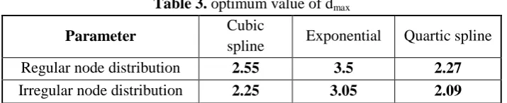
4.2 Size of support domain:

The size of the support domain dmax of the weight function associated to the desired point must be chosen big enough so that the number of points covered by the influence domain guarantees the regularity of matrix A. Very small values can generate big errors when numerical integration based on Gaussian quadrature is used to calculate the array elements of the matrix. On the other hand, dmaxshould be small enough to maintain the local characteristics for the approximation by MLS [5].

Optimum value of domain of influence parameter for end node for different weight function and nodal distribution along the bar are obtained using one point gauss quadrature integration method in MATLAB platform.

Table 3. optimum value of dmax

Parameter Cubic

spline Exponential Quartic spline Regular node distribution 2.55 3.5 2.27 Irregular node distribution 2.25 3.05 2.09

4.3 Order of monomial basis:

Consistency of MLS shape function is controlled by the order of monomial basis (m) function selected for the solution. While constructing MLS shape functions in EFG, order of monomial basis function, PT (x) considered is linear (m=2) and quadratic (m=3) with cubic spline weight function at optimal value of support domain parameter.

0 0.05 0.1 0.15 0.2 0.25 0.3 0.35

0 0.1 0.2 0.3 0.4 0.5 0.6 0.7 0.8 0.9 1

u

Node

efg

Table 4. Effect of Monomial Basis Order (M)

Node Exact

solution m=1 m=2 0.1 0.050 0.0497 0.0498 0.2 0.099 0.0985 0.0988 0.3 0.146 0.1452 0.1456 0.4 0.189 0.189 0.1895 0.5 0.229 0.2287 0.2294 0.6 0.264 0.2635 0.2643

0.7 0.293 0.2922 0.2931 0.8 0.315 0.314 0.315 0.9 0.329 0.3277 0.3295

1 0.333 0.3325 0.3325

4.4 Gauss Quadrature Integration:

Integration cells and number of gauss points are defined over the domain of problem; and it is set by intervals between nodes. High order Gauss quadrature improves solution accuracy but significantly increases the computational efforts. Table 4 shows the effect of 1 point and 2 point gauss quadrature integration for cubic spline weight function with exact solution.

Table 4. Effect of Gauss point

Node Exact solution

1 Gauss point

2 Gauss point 0.1 0.050 0.050 0.050 0.2 0.099 0.099 0.099 0.3 0.146 0.145 0.146 0.4 0.189 0.189 0.189 0.5 0.229 0.229 0.229

0.6 0.264 0.264 0.264 0.7 0.293 0.292 0.293 0.8 0.315 0.314 0.315 0.9 0.329 0.328 0.329

1 0.333 0.333 0.333

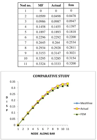
4.5 Comparison of results with FEM:

Table 5 Comparison of EFG with FEM and Analytical Solution

Nod no. MF Actual fem

1 0 0 0

2 0.0509 0.0498 0.0478

3 0.0986 0.0987 0.0947

4 0.1458 0.1455 0.1397

5 0.1897 0.1893 0.1818

6 0.2296 0.2292 0.2200

7 0.2645 0.264 0.2534

8 0.2934 0.2928 0.2811

9 0.3153 0.3147 0.3021

10 0.3295 0.3285 0.3154

11 0.3324 0.3333 0.3200

Figure 6: Comparative Displacement

IV.

CONCLUSION

The meshless methods described in this paper are

especially well-suited for linear elastic problems.

Since standard mesh less methods do not fulfil the

so-called Kronecker–Delta property, essential

boundary conditions cannot be enforced as easily as

in finite element methods and Lagrange multiplier

method. An element free Galerkin (EFG) method

was implemented in MATLAB for linear elastic

problem. The solution by this method seems

accurate enough and converges to the analytical

solution. The EFG method is flexible with respect

to the construction of the shape functions.

Therefore, it is possible to improve the accuracy of

the method by the choice of weight functions and

by the selection of the support domain of EFG

nodes. The results of EFG were found in good

agreement to exact solution than FEM. Uniform

node distribution scheme, Quartic Spline weight

functions and appropriate values of support domain

value and higher number of point in gauss

integration method yield accurate results in EFG

mesh free method.

0 0.05 0.1 0.15 0.2 0.25 0.3 0.35

1 2 3 4 5 6 7 8 9 10 11

D I S P

NODE ALONG BAR

COMPARATIVE STUDY

Meshfree

Actual

V.

REFERENCES

[1]. Liu G. R., 2004, “Mesh Free Methods: moving beyond the finite element method”, Ed. CRC Press, Florida,USA,

[2]. T. Belytschk O, Y.Y.Lu And L.GU, "An Introduction to Programming the Meshless Element Free Galerkin Method" International journal for numerical methods in engineering, VOL. 37, 229-256 (1994).

[3]. T. Belytschko,Y. Krongauz, D. Organ, "Meshless Methods: An Overview and Recent Developments" May 2, 1996.

[4]. J. Dolbow, T. Belytschko, "Numerical integration of the Galerkin weak form in meshfree methods" Computational Mechanics 23 (1999) 219-230 Ó Springer-Verlag 1999.

[5]. S. D. Daxini and J. M. Prajapati, "A Review on Recent Contribution of Meshfree Methods to Structure and Fracture Mechanics Applications" Scientific World Journal Volume 2014, Article ID 247172, 13 pages

[6]. "An Introduction to Meshfree methods and their Programming" by G.R. LIU, 2005.

[7]. "From Weighted Residual Methods
to Finite
Element Methods" by Lars‐Erik Lindgren, 2009.

[8]. "Meshfree and Generalized Finite Element Methods" by Habilitationsschrift, 2008