www.nat-hazards-earth-syst-sci.net/17/563/2017/ doi:10.5194/nhess-17-563-2017
© Author(s) 2017. CC Attribution 3.0 License.
Numerical rainfall simulation with different spatial and temporal
evenness by using a WRF multiphysics ensemble
Jiyang Tian1, Jia Liu1,2, Denghua Yan1, Chuanzhe Li1, and Fuliang Yu1
1State Key Laboratory of Simulation and Regulation of Water Cycle in River Basin, China Institute of
Water Resources and Hydropower Research, Beijing, 100038, China
2State Key Laboratory of Hydrology-Water Resource and Hydraulic Engineering, Hohai University,
Nanjing, 210098, China
Correspondence to:Jia Liu ([email protected])
Received: 3 November 2016 – Discussion started: 6 December 2016
Revised: 17 March 2017 – Accepted: 23 March 2017 – Published: 13 April 2017
Abstract. The Weather Research and Forecasting (WRF) model is used in this study to simulate six storm events in two semi-humid catchments of northern China. The six storm events are classified into four types based on the rainfall evenness in the spatial and temporal dimensions. Two mi-crophysics, two planetary boundary layers (PBL) and three cumulus parameterizations are combined to develop an en-semble containing 16 members for rainfall generation. The WRF model performs the best for type 1 events with rela-tively even distributions of rainfall in both space and time. The average relative error (ARE) for the cumulative rain-fall amount is 15.82 %. For the spatial rainrain-fall simulation, the lowest root mean square error (RMSE) is found with event II (0.4007), which has the most even spatial distribution, and for the temporal simulation the lowest RMSE is found with event I (1.0218), which has the most even temporal distribu-tion. The most difficult to reproduce are found to be the very convective storms with uneven spatiotemporal distributions (type 4 event), and the average relative error for the cumula-tive rainfall amounts is up to 66.37 %. The RMSE results of event III, with the most uneven spatial and temporal distribu-tion, are 0.9688 for the spatial simulation and 2.5327 for the temporal simulation, which are much higher than the other storms. The general performance of the current WRF phys-ical parameterizations is discussed. The Betts–Miller–Janjic (BMJ) scheme is found to be unsuitable for rainfall simula-tion in the study sites. For type 1, 2 and 4 storms, member 4 performs the best. For type 3 storms, members 5 and 7 are the better choice. More guidance is provided for choosing among
the physical parameterizations for accurate rainfall simula-tions of different storm types in the study area.
1 Introduction
Precipitation is a crucial element in the hydrological cycle at regional or global scales. With the characteristics of high intensity, short duration, uneven distribution and sudden oc-currence, the precipitation easily causes floods, with a high peak in semi-humid regions, which is tricky for forecast-ing accurately (Nikolopoulo et al., 2010). The quantitative precipitation forecast (QPF) is an effective method to avoid flood disasters and help flood risk management (Kryza et al., 2013). With the development of computer technology and at-mospheric physics, numerical weather prediction (NWP) has become an efficient method for QPF (Yang et al., 2012).
various physical parameterizations to be applied in differ-ent cases. Each physical parameterization emphasizes on dif-ferent physical processes and has its unique structure and complexity, which may have great influence on the rainfall simulations. That is why numerous sensitivity studies of the WRF parameterizations are carried out in different regions of the world (Klein et al., 2015). Three categories of the pa-rameterizations have been mostly discussed and identified as the main influencing factors for rainfall simulation, i.e., microphysics, planetary boundary layer (PBL) and cumulus parameterizations. Different physical parameterizations are found to be efficient for different rainfall events in different regions (Jankov et al., 2011; Madala et al., 2014; Pennelly et al., 2014).
It is an increasingly difficult task to determine the optimal combination of physical parameterizations due to the devel-opment of the WRF model with more and more choices of parameterizations. Although many studies show that the best physical parameterization combination can be determined by many simulations for a certain rainfall event, it is difficult to tell the characteristics of the future rainfall events for real-time rainfall prediction. In order to consider the uncertainties associated with the selection of physical parameterizations, it has become a common method to use the ensemble in nu-merical rainfall prediction (Evans et al., 2011). Flaounas et al. (2011) studied an ensemble with six members over West Africa, which was produced by two PBL and three cumu-lus parameterizations. An ensemble containing 18 members was investigated in the south-central United States, which was created by three microphysics, three PBL and two cu-mulus parameterizations (Jankov et al., 2005). And an en-semble with 36 members was tested for a series of rainfall events at the south-east coast of Australia, which contained two PBL, two cumulus, three microphysics and three radia-tion parameterizaradia-tions (Flaounas et al., 2011). These studies show that no single physical parameterization combination performs the best for all rainfall events.
In this study, 16 physical parameterization combinations are designed from two microphysics, Purdue–Lin (Lin) and WRF Single-Moment 6 (WSM6), two PBLs, Yonsei Univer-sity (YSU) and Mellor–Yamada–Janjic (MYJ), and three cu-mulus parameterizations, Kain–Fritsch (KF), Grell–Devenyi (GD) and Betts–Miller–Janjic (BMJ). Lin is a sophisticated parameterization which contains five classes of hydromete-ors, and it is suitable for high-resolution simulations (Lin et al., 1983). WSM6 reveals an improvement in the high cloud amount and surface precipitation, which adds graupel micro-physics based on the works of Lin et al. (1983) and Rut-ledge and Hobbs (1983). MYJ PBL is appropriate for all sta-ble or slightly unstasta-ble flows (Janjic, 1994). YSU PBL im-proves the performance of intense convection based on the Medium Range Forecast (MRF) PBL (Hong et al., 2006). KF is a classic cumulus parameterization and has been used successfully for years in many scientific institutions (Kain, 2004). GD is an ensemble cumulus parameterization and can
be used in high resolution models (Grell and Freitas, 2014). BMJ can adjust instabilities in the environment by generating deep convection and has been used extensively throughout the globe (Janjic, 2000).
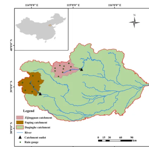
Two medium sized catchments, the Fuping and Zijing-guan, are chosen as the study sites, which are respectively located in the south and the north reaches of the Daqinghe catchment in North China. With the characteristics of high intensity, short duration, uneven distribution and sudden oc-currence, the storm events in the study sites are represen-tative for the semi-humid region with temperate continental monsoon climates. The aim of this study is to determine the potential performance of the WRF model for different types of storm events in semi-humid regions. Six storm events are chosen from the study sites and classified into four differ-ent types based on the rainfall evenness in the spatial and the temporal dimensions. The 16 designed combinations of physical parameterizations are treated as the ensemble for rainfall simulation, and the results regarding both the cumu-lative rainfall amounts and the spatiotemporal patterns are verified.
2 WRF model configuration and designed physical ensemble
in-Figure 1.The nested domains and the orography of the Fuping catchment and Zijingguan catchment.
nermost domain (Skamarock and Klemp, 2008). The time step of the WRF model output is set to 1 h. The spin-up pe-riod is necessary for the WRF model to develop the smaller scale convective features, and the widely used lengths are 6 h (Givati et al., 2012), 12 h (Hu et al., 2010) and 24 h (Wang et al., 2012). Different spin-up lengths were tried for the six storm events in this study, whereas the results did not show obvious differences regarding the simulated rainfall. In order to improve the calculation efficiency for further hydrological use (i.e., flood warning), a 6 h period is chosen to spin up the model. That is to say, the start of the model integration is 6 h earlier than the storm start time, and the end time of the model integration is consistent with the storm end time.
The setting of the WRF model is very important be-fore it is used to simulate the meteorological factors, espe-cially the physical parameterizations. As shown by Table 1, a WRF physical ensemble is constructed by combining dif-ferent choices of the physical parameterizations to simulate the storm events in the study areas. The selection of the pa-rameterizations is based on their good performance in semi-humid regions of China (Givati et al., 2012; Qie et al., 2014; Di et al., 2015). In order to learn the physical parameteri-zations more comprehensively, the different complexity and mechanisms are also considered. WSM6 is the most complex in the series of WSM schemes, which is revised based on Lin (Hong and Lim, 2006). YSU is a non-local closure scheme, while MYJ is a local closure scheme (Evans et al., 2011). The KF is a simple cloud model which can be triggered when air parcel temperature at its lifting condensation level is larger than the environmental air (Pennelly et al., 2014). The GD
Table 1.The constitution of the WRF physical ensemble.
Ensemble Microphysics PBL Cumulus
ID parameterization
1 Lin YSU KF
2 WSM6 YSU KF
3 Lin MYJ KF
4 WSM6 MYJ KF
5 Lin YSU GD
6 WSM6 YSU GD
7 Lin MYJ GD
8 WSM6 MYJ GD
9 Lin YSU BMJ
10 WSM6 YSU BMJ
11 Lin MYJ BMJ
12 WSM6 MYJ BMJ
13 Lin YSU /
14 WSM6 YSU /
15 Lin MYJ /
16 WSM6 MYJ /
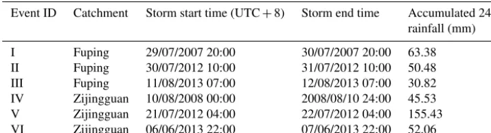
3 Storm events and evaluation statistics 3.1 Study area and storm events
The Fuping and Zijingguan catchments are the study areas, which respectively belong to the south and north reaches of the Daqinghe catchment, located in northern China with semi-humid climatic conditions. The drainage area of Fup-ing (from lat 39◦220 to 38◦470N and from long 113◦400 to 114◦180E) is 2210 km2, and the area of Zijingguan (from lat 39◦130 to 39◦400N and from long 114◦280 to 115◦110E) is 1760 km2(shown by Fig. 2). The average annual rainfall is about 600 mm at the study sites, and the majority of rain fo-cuses in the flood season. As shown by Fig. 2, there are eight rain gauges in the Fuping catchment and 11 rain gauges in the Zijingguan catchment. The observed hourly rainfall data from rain gauges are treated as the ground truth. Six 24 h storm events are selected from the 10 recent years (2006 to 2015) with the respective rainfall characteristics of the study sites. The encounter between the western pacific subtropical high and the cold vortex of westerlies and the strong upward motion caused by Taihang Mountains are the main factors of rain formation in the study area, while the six storm events have quite different spatial and temporal evenness. Table 2 shows the duration and accumulative rainfall amounts of the six storm events.
The six storm events are categorized into four types based on the rainfall evenness of the spatiotemporal distribution (Liu et al., 2012). The variation coefficientCvis used to
eval-uate the uneven level:
Cv= v u u t
1 N
N X
i=1
(xi x −1)
2. (1)
Figure 2. The location of the Daqinghe catchment in northern China (light shading) and the locations of the two study sites in the Daqinghe catchment.
For the spatial distribution, xi is the 24 h rainfall
accumu-lation at rain gaugei, andx is the average ofxi; N is the
number of rain gauges. For the temporal distribution,xi is
the hourly areal rainfall at timei, andx is the average ofxi;
Nis the number of hours.
The higherCv is, the more uneven the rainfall is. In
or-der to learn the spatial and temporal evenness of the rain-fall in the two catchments, both spatial and temporalCv of
the storm events from 1985 to 2015 are calculated. In real-ity, rainfall in northern China is much more uneven than the south, and it is impossible to find absolute even rainfall in both space and time. Therefore, we chose a threshold of 5 %, which is also considered in other statistical analyses in the same area, as the critical value to separate even and uneven rainfall events. With the threshold, we found the two criti-cal values of 0.4 for the spatialCvand 0.6 for the temporal
Cv. That is to say, the storm events with a spatialCvbelow
0.4 or with a temporalCvbelow 1.0 account for 5 % of the
total storm events from 1985 to 2015 in the study area. Ta-ble 3 shows the spatial and temporalCvof observations for
Table 2.Durations and rainfall accumulations of the six selected 24 h storm events.
Event ID Catchment Storm start time (UTC+8) Storm end time Accumulated 24 h rainfall (mm)
I Fuping 29/07/2007 20:00 30/07/2007 20:00 63.38
II Fuping 30/07/2012 10:00 31/07/2012 10:00 50.48
III Fuping 11/08/2013 07:00 12/08/2013 07:00 30.82
IV Zijingguan 10/08/2008 00:00 2008/08/10 24:00 45.53 V Zijingguan 21/07/2012 04:00 22/07/2012 04:00 155.43 VI Zijingguan 06/06/2013 22:00 07/06/2013 22:00 52.06
Table 3.Spatial and temporalCvof the observed rainfall for the six storm events.
Indices Type 1 Type 2 Type 3 Type 4
Event I Event II Event VI Event IV Event V Event III
SpatialCv 0.3975 0.1927 0.3258 0.4588 0.6098 0.7400 TemporalCv 0.6011 1.0823 1.8865 1.3779 1.8865 2.3925
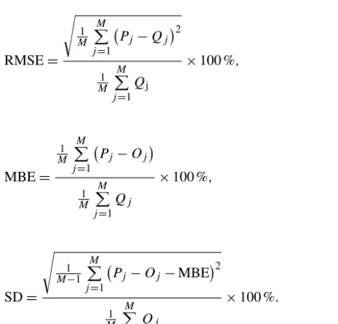
3.2 Verification indices for rainfall simulations
For evaluating the accuracy of rainfall simulation, both the accumulated areal rainfall and the spatiotemporal distribu-tion of the rainfall are important. The accumulated areal rain-fall is evaluated by the relative error (RE):
RE=(P−Q)
Q ×100 %, (2)
whereP is the simulated value, which is the average value of all the grids inside the study area, andQis the observed value, which is calculated by the Thiessen polygon method based on the observations of the rain gauges (Sivapalan and Blöschl, 1998; Jarvis et al., 2013).
The spatial and temporal distributions of the rainfall are evaluated by a two-dimensional verification scheme. Both in spatial and temporal dimensions, some categorical and con-tinuous indices are selected and calculated (Liu et al., 2012). The categorical verification indices are chosen as the prob-ability of detection (POD), the frequency bias index (FBI), the false alarm ratio (FAR) and the critical success index (CSI). The calculation of the categorical indices depends on whether it rains or not, as shown in Table 4. It should be mentioned that the insignificant precipitation (less than 0.1 mm h−1) is regarded as no rain. For verification in the spatial dimension, the comparison is made between the ob-servations of the rain gauges and the simulations of the WRF model at each time step i, and then the average values are calculated by the categorical indices at all the time steps for the final results. As shown by the Eqs. (3)–(6),N is the to-tal number of time steps of the WRF model output, which is 24 in this study. For the temporal dimension, the time series data of simulation and observation are used to calculate the four indices at each rain gaugei, then the average values are calculated by the indices at all the rain gauges for the final
results. This timeN is the number of the rain gauges of the Fuping and Zijingguan catchments respectively in Eqs. (3)– (6).
POD= 1
N
N X
i=1
NAi
NAi+NCi
, (3)
FBI= 1
N
N X
i=1
NAi+NBi
NAi+NCi
, (4)
FAR= 1
N
N X
i=1
NBi
NAi+NBi
, (5)
CSI= 1
N
N X
i=1
NAi
NAi+NBi+NCi
. (6)
For the four categorical indices, POD indicates the per-centage of correct simulation for the observed rainfall. FBI shows whether the WRF model has a tendency to overes-timate (FBI > 1) or underesoveres-timate (FBI < 1) rainfall occur-rences, while FBI cannot show closeness of the simulation and the observation. FAR represents the ratio of false alarms, and CSI indicates the percentage of correct simulation be-tween the simulated and observed rainfall. The perfect scores of POD, FBI, FAR and CSI are 1, 1, 0 and 1, respectively.
Table 4.Rain–no rain contingency table for the WRF simulation against observation.
WRF/observations Rain No rain
Rain NA (hit) NB (false alarm)
No rain NC (failure) ND (correct negative)
continuous indices are expressed by Eqs. (7)–(9).
RMSE= s 1 M M P
j=1
Pj−Qj2
1 M
M P
j=1
Qj
×100 %, (7)
MBE=
1 M
M P
j=1
Pj−Oj
1 M
M P
j=1
Qj
×100 %, (8)
SD=
s 1 M−1
M P
j=1
Pj−Oj−MBE 2
1 M
M P
j=1
Qj
×100 %. (9)
For the spatial dimension,Pj andQj are the simulation and
observation of 24 h rainfall accumulations at each rain gauge j.Mis the number of the rain gauges, which is 8 for the Fup-ing catchment and 11 for the ZijFup-ingguan catchment. For the temporal dimension,PjandQjare the average areal rainfall
simulation and observation at each time stepj. This timeM is 24, which represents the number of the time steps. The fi-nal values of the three indices represent the mean magnitude of error, the average cumulative error and the variation of the simulation error of MBE, respectively. The perfect score of all the three indices is 0. In order to compare the simulations for different storm events, the final values of the three con-tinuous indices in both two dimensions are represented as percentages of the corresponding average observations.
4 Results
4.1 Simulations of the 24 h rainfall accumulations The simulation results of the cumulative rainfall amounts from the 16 members of the physical ensemble are shown in Table 5 and ranked according to REs. Members 5, 4 and 2 rank in the top three for event I (storm type 1), with rela-tively lower REs. For type 2 events, members 4 and 12 show more stable performances, ranking in the top five for both
events II and VI. For type 3 events, members 5 and 7 are better choices, with top 5 rankings for events IV and V. The top four members for event III (type 4) are members 4, 2, 16 and 3. It can be seen that the performances of the 16 mem-bers are quite distinct for different types of storm events. In addition, the difference among the 16 members varies signif-icantly for a certain storm event. For example, the difference of REs for member 8 (18.44 %) and member 9 (−37.69 %) reaches up to 56.13 % for event I. While for event V, the largest difference of RE among all the 16 members is only 9.10 %. There are great uncertainties for the simulation of the different storm events using the WRF model with differ-ent combinations of the physical parameterizations. It’s hard to tell which parameterization combination is the best, but only to find the one with the best general performance. In this study, member 4 could be the best choice considering its stable top rankings for storm types 1, 2 and 4, while mem-bers 9, 10, 11 and 12 have a worse performance for storm types 1 and 4. For type 3 events, members 5 and 7 are better choices. However, in real-time rainfall prediction, there is a necessity to use a physical ensemble since it is always tricky to tell the exact characteristics of the future storm before it happens, and the use of a determined combination of param-eterizations which performs generally well cannot always lead to the best results. According to Table 5, the four mem-bers without cumulus parameterization have a quite different performance for different events. For example, member 15 performs the best for event IV; nevertheless, it performs the worst for event V. Comparing the members containing cu-mulus parameterization, members 13, 14, 15 and 16 have no significant advantages or significant disadvantages for rain-fall simulation. Taking event I as an example, the best one (member 16) of the 4 members without cumulus parameter-ization ranks 4th out of the 16 members, whereas the worst one (member 13) ranks 12th. However, few members without cumulus parameterization rank in the top four, which means that it is necessary to use cumulus parameterization for the simulation of rainfall accumulation.
Table 5.Rankings of the 16 members of the physical ensemble according to RE (%) of the simulated rainfall accumulations for the storm events.
Ranking Type 1 Type 2 Type 3 Type 4
I II VI IV V III
1 Member 5
(−0.17)
Member 8 (−24.05)
Member 3 (−16.32)
Member 15 (−21.89)
Member 10 (−57.89)
Member 4 (−42.41)
2 Member 4
(3.85)
Member 12 (−25.12)
Member 4 (−17.03)
Member 5 (−25.77)
Member 2 (−58.91)
Member 2 (−45.35)
3 Member 2
(7.23)
Member 4 (−29.12)
Member 1 (−33.05)
Member 7 (−27.03)
Member 7 (−59.22)
Member 16 (−46.55)
4 Member 16
(−7.47)
Member 10 (−30.09)
Member 2 (−38.87)
Member 16 (−27.13)
Member 1 (−59.31)
Member 3 (−46.93)
5 Member 6
(10.17)
Member 6 (−30.72)
Member 12 (−45.79)
Member 6 (−32.19)
Member 5 (−59.54)
Member 15 (−47.59)
6 Member 1
(10.55)
Member 14 (−32.10)
Member 11 (−46.60)
Member 13 (−32.43)
Member 12 (−59.57)
Member 1 (−48.59)
7 Member 15
(−10.99)
Member 7 (−32.23)
Member 7 (−51.66)
Member 9 (−33.17)
Member 4 (−60.15)
Member 7 (−69.79)
8 Member 14
(−10.83)
Member 2 (−33.27)
Member 5 (−52.76)
Member 8 (−33.90)
Member 11 (−60.20)
Member 8 (−70.95)
9 Member 7
(13.96)
Member 15 (−33.36)
Member 8 (−53.12)
Member 11 (−36.23)
Member 9 (−60.24)
Member 13 (−73.88)
10 Member 3
(17.54)
Member 16 (−34.03)
Member 6 (−54.57)
Member 1 (−37.53)
Member 6 (−60.81)
Member 14 (−77.06)
11 Member 8
(18.44)
Member 11 (−34.59)
Member 15 (−56.48)
Member 10 (−39.93)
Member 3 (−61.17)
Member 5 (−77.19)
12 Member 13
(−20.12)
Member 3 (−39.71)
Member 10 (−57.85)
Member 14 (−40.24)
Member 14 (−62.37)
Member 6 (−78.70)
13 Member 10
(−22.63)
Member 13 (−39.72)
Member 16 (−58.78)
Member 3 (−42.64)
Member 8 (−62.43)
Member 10 (−81.42)
14 Member 11
(−27.30)
Member 9 (−40.24)
Member 9 (−59.85)
Member 12 (−42.99)
Member 13 (−65.12)
Member 9 (−83.77)
15 Member 12
(−34.24)
Member 5 (−40.41)
Member 13 (−63.66)
Member 4 (−51.58)
Member 16 (−65.73)
Member 11 (−85.16)
16 Member 9
(−37.69)
Member 1 (−42.15)
Member 14 (−65.04)
Member 2 (−53.36)
Member 15 (−66.99)
Member 12 (−86.59)
rainfall occurrences always keep step with the observations. While for events IV, V and III (type 3 and type 4 events), the simulated starting and ending times of the rainfall du-rations are quite different from the observations. It can be determined that type 1 and type 2 events have even rainfall distributions in space, while the spatial rainfall is unevenly distributed in space for type 3 and type 4 events. It seems that storms with rainfall evenly distributed in space tend to have better simulation results in the temporal patterns of rainfall accumulations.
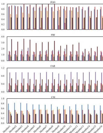
4.2 Simulations of the spatial rainfall distributions
In order to compare the simulation results of the different storm types in detail, seven verification indices are first calcu-lated to evaluate the simucalcu-lated rainfall distributions in space. Figures 4 and 5 respectively show the values of the
categor-Table 6.AREs of the 16 members of the physical ensemble for the four types of storm events (%).
Type 1 Type 2 Type 3 Type 4
I II VI IV V III
15.82 33.80 43.96 48.22 64.18 66.37
ical indices and continuous indices for the six storm events with the 16 members of the physical ensemble.
Figure 3.Cumulative curves of the observed and simulated areal rainfall for the six storm events.
the 16 members for type 4 event (event III) are all close to zero, indicating that the WRF model can hardly capture the storm occurrence in space. Events I and IV have nearly per-fect scores of FBI, which are close to 1.0. For events II, III and VI, WRF tends to overestimate the rainfall occurrences,
0.0 0.2 0.4 0.6 0.8
1.0 POD
0.0 1.0 2.0 3.0
4.0 FBI
0.0 0.4 0.8
1.2 FAR
0.0 0.2 0.4 0.6 0.8
1.0 CSI
Event I Event II Event III Event IV Event V Event VI
Figure 4.Spatial values of the four categorical indices for different storm events with the 16 members of the physical ensemble.
in space because of the high FARs (near 1.0). Storm type 3 outperforms storm type 2, with relatively lower FARs. CSI can be considered as a comprehensive description of accu-racy. Storm type 1, with the highest CSIs, performs the best of all the 16 members, while CSIs of storm type 4 are all close to zero, showing that the simulation results are unreli-able. CSIs of the other two storm types have few differences as a whole, but the index values are a little bit higher for events with more evenly distributed rainfall in space.
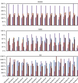
Figure 5 shows that the values of RMSE have great change in different members for a certain event. RMSE is always re-garded as the key quantitative index to estimate errors. Storm event II, with the lowest Cv, always has the lowest RMSE
for the 16 members, which means that the WRF model
mem-0 % 20 % 40 % 60 % 80 %
100 % RMSE
0 % 20 % 40 % 60 % 80 % 100 %
120 % MBE
0 % 20 % 40 % 60 % 80 %
100 % SD
Event I Event II Event III Event IV Event V Event VI
Figure 5.Spatial values of the three continuous indices for different storm events with the 16 members of the physical ensemble.
bers, which indicates that there are always some members performing better than the 4 members without cumulus rameterization. It is helpful to use appropriate cumulus pa-rameterization for the simulation of the spatial rainfall distri-bution.
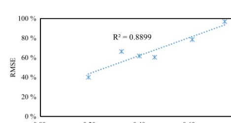
The average values of the 16 members for all the seven indices are calculated to quantitatively analyze the perfor-mance of the WRF model in spatial dimension for the four storm types. As shown in Table 7, the value of POD for storm type 1 is higher than storm types 3 and 4. In addition, the value of CSI for storm type 1 is the highest, and the value of FAR is the lowest in the four storm types. The lower values of RMSE and MBE for storm type 1 also indicate that the WRF model performs well for storm type 1. The simulations of type 3 events are worse than type 2 events, showing lower POD and higher RMSE values, though the FARs of the type 2 events are a little higher than type 3 events. The lowest POD and CSI and the highest FAR and RMSE can be found with storm type 4, which indicates that the WRF model can hardly capture this kind of storm accurately in space. Since the in-dex of RMSE shows the actual magnitude of errors without canceling out the positive and negative errors, a correlation
R² = 0.8899
0 % 20 % 40 % 60 % 80 % 100 %
0.00 0.20 0.40 0.60 0.80
R
M
SE
Cv
Figure 6.The relationship between RMSE and Cv in the spatial dimension.
analysis is further carried out between RMSE and the spatial evenness indicatorCv. It’s interesting to find that RMSE and
Cvhave a good linear relationship and the correlation
Table 7.Average index values of the 16 members of the physical ensemble for the simulations of the spatial rainfall distributions.
Types of storm events Categorical indices Continuous indices (%)
POD FBI FAR CSI RMSE MBE SD
Type 1 Event I 0.8440 0.9815 0.1313 0.7565 61.74 21.21 53.54 Type 2 Event II 0.8934 1.5877 0.4238 0.5357 40.07 35.67 15.74 Event VI 0.9014 2.8866 0.6187 0.3516 66.36 42.74 49.78 Type 3 Event IV 0.6460 0.9974 0.3285 0.4873 60.46 45.49 41.10 Event V 0.4671 0.6906 0.3215 0.3821 78.65 61.51 51.36 Type 4 Event III 0.0503 1.6301 0.9731 0.0194 96.88 66.14 63.53
0.0 0.2 0.4 0.6 0.8
1.0 POD
0.0 1.0 2.0 3.0 4.0
5.0 FBI
0.0 0.3 0.6 0.9
1.2 FAR
0.0 0.2 0.4 0.6 0.8
1.0 CSI
Event I Event II Event III Event IV Event V Event VI
0 % 50 % 100 % 150 % 200 % 250 %
300 % RMSE
0 % 20 % 40 % 60 % 80 %
100 % MBE
0 % 200 % 400 % 600 % 800 % 1000 %
1200 % SD
Event I Event II Event III Event IV Event V Event VI
Figure 8.Temporal values of the three continuous indices for different storm events with the 16 members of the physical ensemble.
4.3 Simulations of the temporal rainfall patterns
The seven indices are also calculated in the temporal dimen-sion to evaluate the simulated rainfall patterns in time. The values are respectively shown in Figs. 7 and 8. In Fig. 7, PODs of storm types 1 and 2 are all above 0.70 and much higher than storm types 3 and 4 in the 16 members. It in-dicates that storm types 1 and 2 can be accurately simulated with regards to the rainfall occurrence in the temporal dimen-sion, while the WRF model fails with storm type 4, with all PODs of the 16 members close to 0. For FBI, the scores of events I and IV are nearly perfect, but the other four events show tendencies of overestimating the rainfall occurrences in time, especially event VI. The lowest FAR values are also found with storm type 1, with all the values less than 0.20 in the 16 members. Storm type 4 has the highest FARs, which are close to 1.0 in some members. Based on the FAR index, the ranking of the WRF performance in simulating tempo-ral rainfall occurrences is type 1 > type 3 > type 2 > type 4, from the best to the worst. In the 16 members, CSIs of storm type 1 are always the highest, while CSIs of storm type 4 are
always the lowest. It should be mentioned that the CSI is 0 in members 7, 11, 14 and 15 in storm event III, indicating a bad simulation of the temporal rainfall occurrences for this type 4 event.
nec-essary to use cumulus parameterization for the simulation of the temporal rainfall distribution.
The average ensemble values for the seven indices are also calculated for evaluating the performance of the WRF model in simulating the temporal rainfall patterns. The results are shown in Table 8. The values of POD and CSI for storm type 1 are the highest, and the values of FAR and RMSE are the lowest in the four storm types, which indicate that the WRF model performs best for storm type 1. The model per-forms the worst for storm type 4, with the lowest POD and CSI and the highest FAR and RMSE. In general, the simula-tion results of the temporal rainfall patterns are unsatisfactory for all the four storm types. The linear relationship between RMSE and the temporalCvis also significant and the
corre-lation coefficient of linear regression (R2)is 0.7524 (shown by Fig. 9). It indicates that the simulation error also increases with the increase of the rainfall unevenness in the temporal dimension.
5 Discussion
In this study, the performances of 16 WRF physical mem-bers are estimated firstly by AREs for cumulative rainfall amounts and then by a two-dimensional verification scheme for spatiotemporal rainfall distributions. According to the spatiotemporal evenness, six storm events are classified into four storm types. Storm type 1 has a two-dimensional even-ness of rainfall which is even in the spatiotemporal distri-bution. The WRF model performs best for simulating this storm type, not only for the cumulative rainfall amounts but also for the spatiotemporal distributions. Storm type 2 is only even in space, and the simulation results from the WRF en-semble are better than storm types 3 and 4. But compared with type 1, the cumulative rainfall amounts of type 2 events are seriously underestimated. Storm types 3 and 4 are both uneven in spatiotemporal distribution, and the unevenness is especially remarkable for type 4 events. The simulations of the WRF model are unsatisfactory for the spatiotempo-ral patterns of the two storm types. The simulation results of type 4 events are the worst among the four storm types. Some of the members even miss the whole storm duration in space and time. It is interesting to find that the WRF model tends to underestimate the rainfall amounts except for storm type 1. With more events being investigated in the study sites, the general simulation errors of the WRF model can be de-termined by statistical analysis, which can help build a cor-rection model to further improve the rainfall products of the WRF model.
For rainfall forecast operation, it is hard to identify the storm type before the storm occurs. Therefore it is impor-tant to determine the physical parameterizations which gen-erally perform well. According to the REs of the 16 mem-bers for the six storm events shown in Table 5, the AREs of the six storm events for one certain member are
cal-R² = 0.7524
0 % 50 % 100 % 150 % 200 % 250 % 300 %
0.00 0.50 1.00 1.50 2.00 2.50 3.00
R
M
SE
Cv
Figure 9.The relationship between RMSE andCvin the temporal dimension.
culated. It is interesting to find that members containing BMJ have relatively higher AREs, which are 52.49 % (mem-ber 9), 48.30 % (mem(mem-ber 10), 48.35 % (mem(mem-ber 11) and 49.05 % (member 12) respectively. The relative lower AREs (34.02–39.50 %) can be found in members which contain KF. The members containing GD perform better than members with BMJ while worse than members with KF. The range of the AREs is 42.32–44.53 %. The members without cumu-lus parameterization also perform better than members with BMJ while worse than members with KF, and the range of the AREs is 39.55–49.16 %. That is to say, the cumulus pa-rameterizations have a significant effect on the performance of the WRF model and BMJ performs the worst in the three cumulus parameterizations. Janjic (2000) indicated that BMJ performed poorly in accurately reproducing the range and the intensity of the low-level jet. The strong ability of BMJ in simulating the upward transportation of vapor always results in underestimation of the rainfall amount. That is the main reason why BMJ is not a good choice in the study area. Ad-ditionally, it is necessary to use cumulus parameterization for the simulation of the rainfall accumulation and spatiotempo-ral rainfall distribution in the study area. However, the thresh-old of the horizontal resolution needs to be further discussed to determine whether to use the cumulus parameterization.
The uncertainties of the rainfall processes affect the choice of the physical parameterizations in a certain area. It is nec-essary to select the most appropriate physical parameteriza-tions to design the physical ensemble for rainfall simulation and prediction. In this study, the 16 members of the physical ensemble are constituted from two microphysics, two PBL and three cumulus parameterizations, which are proven to be appropriate and widely used in the neighboring areas of the study sites (Hong et al., 2006; Miao et al., 2011; Pan et al., 2014). With the development of the WRF model, more so-phisticated and realistic physical parameterizations could be developed and should be tested in the study area.
simula-Table 8.Average index values of the 16 members of the physical ensemble for the simulations of the temporal rainfall patterns.
Types of storm events Categorical indices Continuous indices (%)
POD FBI FAR CSI RMSE MBE SD
Type 1 Event I 0.8341 1.0389 0.1621 0.7264 102.18 −20.37 805.67 Type 2 Event II 0.8531 2.9596 0.4654 0.5153 116.27 −37.74 236.57 Event VI 0.8044 3.5119 0.7310 0.2527 161.29 −45.55 787.85 Type 3 Event IV 0.5683 0.8429 0.2931 0.3894 167.89 −43.11 650.35 Event V 0.4083 1.6646 0.2880 0.2947 140.00 −65.60 812.78 Type 4 Event III 0.0427 2.1653 0.9040 0.0148 253.27 −66.08 948.23
tions in both the spatial and the temporal dimension is used. It is assumed that the observations from rain gauges are ac-curate and representative for the two study sites. However, it brings uncertainties to use point-based observations to eval-uate grid-based simulations. More grid-based observational data should be involved to improve the reliability of evalua-tion, especially those from weather radar and remote sensing. Ultimately, the main goal of rainfall forecasts is to ob-tain efficient flood forecasts. The peak flood, flood peak ap-pearance time and flood process are all significantly influ-enced by the rainfall accumulations and the spatiotemporal distribution of the rainfall (Schellekens et al., 2011; Cane et al., 2013; Fan et al., 2015). Event V, which occurred on 21 July 2012, has caused the greatest flood during the past 10 years in Jing-Jin-Ji (Beijing–Tianjin–Hebei) area and re-ceived widespread attention in China. The 24 h rainfall accu-mulation was 155.43 mm in the Zijingguan catchment, and the peak flow reached 2580 m3s−1at the catchment outlet. In such cases, accurate rainfall simulations and predictions can greatly help flood warnings. However, to analyze the useful-ness of the WRF simulations to flood warning, the rainfall– runoff transformation processes should be further consid-ered. This will involve many uncertainties, such as the choice of the rainfall–runoff model, the data used for model cali-bration and the involvement of a real-time updating scheme, which also has a considerable impact on the accuracy of the flood forecasting results. The exploration of different param-eterizations for flood warning purposes is an important issue and worth discussing in further study.
6 Conclusion
In this study, the FNL data from NCAR provide the initial and boundary conditions for the WRF model, which is used for rainfall simulation of six representative storm events with a duration of 24 h in the Fuping and Zijingguan catchments, located in the south and the north reaches of the Daqinghe basin in semi-humid areas of North China. Two micro-physics, two PBL and three cumulus parameterizations are selected to develop the 16 members of the physical ensem-ble of the WRF model. Both the cumulative amount and the
spatiotemporal patterns of the simulated rainfall are analyzed and verified. The relative error is used to evaluate the 24 h ac-cumulated areal rainfall. The spatial rainfall distributions and temporal rainfall patterns are verified by a two-dimensional verification scheme including four categorical and three con-tinuous indices. The six storm events are classified into four types based on the spatiotemporal evenness of the rainfall. In general, the ranking of the average model performance for different storm types is type 1 > type 2 > type 3 > type 4, from the best to the worst, depending on both the cumulative rain-fall amounts and the spatiotemporal rainrain-fall patterns. A nega-tive correlation is found between the simulation error and the rainfall evenness in both spatial and temporal dimensions. Storm events with more evenly distributed rainfall tend to have better simulation results in space and time. In addition, for the small catchment scale, accumulated areal rainfall is more important than the spatiotemporal rainfall distributions. According to the REs of rainfall accumulations, member 4 is the better choice for storm types 1, 2 and 4, while mem-bers 9, 10, 11 and 12 have the worse performance for storm types 1 and 4. For type 3 events, members 5 and 7 are the bet-ter choices. It provides a reference for choosing the optimal ensemble in the study area for different storm types.
Data availability. The observed rainfall data have been obtained from the rain gauges in the Fuping catchment and the Zijingguan catchment. The rain gauges are operated by the Bureau of Wa-ter Resources Survey of Hebei, and the observed rainfall data are also kindly provided by the Bureau of Water Resources Survey of Hebei (Bureau of Water Resources Survey of Hebei, 2006–2015). The global analysis data (FNL) are provided by the National Cen-ters for Environmental Prediction (NCEP, 2007–2013). For access to the FNL data, please contact NCEP.
Author contributions. All the authors have contributed to the
con-ception and development of this manuscript. Jiyang Tian carried out the analysis and wrote the paper. Jia Liu and Fuliang Yu conceived and designed the framework. Denghua Yan and Chuanzhe Li pro-vided assistance in calculations and figure production.
Competing interests. The authors declare that they have no conflict
of interest.
Acknowledgements. This study was supported by the National
Natural Science Foundation of China (grant no. 51409270), the National Key Research and Development Project (grant no. 2016YFA0601503), the International Science and Technology Cooperation Program of China (grant no. 2013DFG70990), the Foundation of China Institute of Water Resources and Hydropower Research (1232) and the Open Research Fund Program of State Key Laboratory of Hydrology-Water Resources and Hydraulic Engineering (2014490611).
Edited by: R. Trigo
Reviewed by: two anonymous referees
References
Aligo, E. A., Gallus, W. A., and Segal, M.: On the im-pact of WRF model vertical grid resolution on Midwest summer rainfall forecasts, Weather Forecast., 24, 575–594, doi:10.1175/2008WAF2007101.1, 2009.
Argüeso, D., Hidalgomuñoz, J. M., Gámizfortis, S. R., Esteban-parra, M. J., Dudhia, J., and Castrodiez, Y.: Evaluation of WRF parameterizations for climate studies over Southern Spain using a multistep regionalization, J. Climate, 24, 5633–5651, doi:10.1175/JCLI-D-11-00073.1, 2011.
Bruno, F., Cocchi, D., Greco, F., and Scardovi, E.: Spatial recon-struction of rainfall fields from rain gauge and radar data, Stoch. Environ. Res. Risk Assess., 28, 1235–1245, doi:10.1007/s00477-013-0812-0, 2014.
Bureau of Water Resources Survey of Hebei: Observed rainfall data from rain gauges, available at: http://www.hbsw.net/, 2006– 2015.
Cane, D., Ghigo, S., Rabuffetti, D., and Milelli, M.: Real-time flood forecasting coupling different postprocessing techniques of precipitation forecast ensembles with a distributed hydro-logical model. The case study of may 2008 flood in western
Piemonte, Italy, Nat. Hazards Earth Syst. Sci., 13, 211–220, doi:10.5194/nhess-13-211-2013, 2013.
Cardoso, R. M., Soares, P. M., Miranda, P. M. A., and Belo-Pereira, M.: WRF high resolution simulation of Iberian mean and ex-treme precipitation climate, Int. J. Climatol., 33, 2591–2608, doi:10.1002/joc.3616, 2013.
Chambon, P., Zhang, S. Q., Hou, A. Y., Zupanski, M., and Che-ung, S.: Assessing the impact of pre-GPM microwave precip-itation observations in the Goddard WRF ensemble data as-similation system, Q. J. Roy. Meteor. Soc., 140, 1219–1235, doi:10.1002/qj.2215, 2014.
Chen, F., Liu, C., Dudhia, J., and Chen, M.: A sensitivity study of high-resolution regional climate simulations to three land surface models over the western United States, J. Geophys. Res., 119, 7271–7291, doi:10.1002/2014JD021827, 2014.
Collischonn, W., Haas, R., Andreolli, I., and Tucci, C. E. M.: Forecasting River Uruguay flow using rainfall forecasts from a regional weather-prediction model, J. Hydrol., 305, 87–98, doi:10.1016/j.jhydrol.2004.08.028, 2005.
Di, Z., Duan, Q., Wei, G., Chen, W., Gan, Y. J., Quan, J., Li, j., Miao, C., Ye, A., and Tong, C.: Assessing WRF Model Param-eter Sensitivity: A Case Study with 5-day Summer Precipitation Forecasting in the Greater Beijing Area, Geophys. Res. Lett., 42, 579–587, doi:10.1002/2014GL061623, 2015.
Evans, J. P., Ekström, M., and Ji, F.: Evaluating the performance of a WRF physics ensemble over South-East Australia, Clim. Dy-nam., 39, 1241–1258, doi:10.1007/s00382-011-1244-5, 2011. Fan, F. M., Collischonn, W., Quiroz, K. J., Sorribas, M. V., Buarque,
D. C., and Siqueira, V. A.: Flood forecasting on the Tocantins River using ensemble rainfall forecasts and real-time satellite rainfall estimates, J. Flood Risk Manag., 9, 278–288, 2015. Flaounas, E., Bastin, S., and Janicot, S.: Regional climate
mod-elling of the 2006 West African monsoon: sensitivity to convec-tion and planetary boundary layer parameterizaconvec-tion using WRF, Clim. Dynam., 36, 1083–1105, doi:10.1007/s00382-010-0785-3, 2011.
Givati, A., Lynn, B., Liu, Y., and Rimmer, A.: Using the WRF Model in an Operational Streamflow Forecast System for the Jordan River, J. Appl. Meteorol. Clim., 51, 285–299, doi:10.1175/JAMC-D-11-082.1, 2012.
Grell, G. A. and Freitas, S. R.: A scale and aerosol aware stochastic convective parameterization for weather and air quality model-ing, Atmos. Chem. Phys., 14, 5233–5250, doi:10.5194/acp-14-5233-2014, 2014.
Guo, X., Fu, D., Guo, X., and Zhang, C.: A case study of aerosol impacts on summer convective clouds and pre-cipitation over northern China, Atmos. Res., 142, 142–157, doi:10.1016/j.atmosres.2013.10.006, 2014.
Ha, J. H. and Lee, D. K.: Effect of Length Scale Tuning of Back-ground Error in WRF- 3DVAR System on Assimilation of High-Resolution Surface Data for Heavy Rainfall Simulation, Adv. Atmos. Sci., 29, 1142–1158, doi:10.1007/s00376-012-1183-z, 2012.
Hong, S. Y. and Lim, J. O. J.: The WRF Single-Moment 6-Class Microphysics Scheme (WSM6), J. Korean Meteorol. Soc., 42, 129–151, 2006.
Hong, S. Y., Noh, Y., and Dudhia, J.: A new vertical diffusion pack-age with an explicit treatment of entrainment processes, Mon. Weather Rev., 134, 2318–2341, doi:10.1175/MWR3199.1, 2006. Hu, X. M., Nielsengammon, J. W., and Zhang F.: Evalu-ation of three planetary boundary layer schemes in the WRF model, J. Appl. Meteorol. Clim., 49, 1831–1844, doi:10.1175/2010JAMC2432.1, 2010.
Janjic, I. Z.: The step-mountain eta coordinate model: Further developments of the convection, viscous sublayer, and tur-bulence closure schemes, Mon. Weather Rev., 122, 927–945, doi:10.1175/1520-0493(1994)122<0927:TSMECM>2.0.CO;2, 1994.
Jankov, I., Gallus, W. A., Swgal, M., and Koch, S. E.: The impact of different WRF model physical parameterizations and their in-teractions on warm season MCS rainfall, Weather Forecast., 20, 1048–1060, doi:10.1175/WAF888.1, 2005.
Jankov, I., Grasso, L. D., Senguota, M., Neiman, P. J., Zupanski, D., Zupanski, M., Lindsey, D., Hillger, D. W., Birkenheuer, D. L., Brummer, R., and Yuan, H.: An evaluation of five ARW-WRF microphysics schemes using synthetic GOES imagery for an at-mospheric river event affecting the California coast, J. Hydrom-eteorol., 12, 618–633, doi:10.1175/2010JHM1282.1, 2011. Jarvis, D., Stoeckl, N., and Chaiechi, T.: Applying
economet-ric techniques to hydrological problems in a large basin: Quantifying the rainfall–discharge relationship in the Bur-dekin, Queensland, Australia, J. Hydrol., 496, 107–121, doi:10.1016/j.jhydrol.2013.04.043, 2013.
Kain, J. S.: The Kain Fritsch convective parameterization: an update, J. Appl. Meteorol., 43, 170–181, doi:10.1175/1520-0450(2004)043<0170:TKCPAU>2.0.CO;2, 2004.
Klein, C., Heinzeller, D., Bliefernicht, J., and Kunstmann, H.: Variability of West African monsoon patterns generated by a WRF multi-physics ensemble, Clim. Dynam., 45, 1–23, doi:10.1007/s00382-015-2505-5, 2015.
Kryza, M., Werner, M., Walaszek, K., and Dore, A. J.: Application and evaluation of the WRF model for high-resolution forecasting of rainfall – a case study of SW Poland, Meteorol. Z., 22, 595– 601, doi:10.1127/0941-2948/2013/0444, 2013.
Lee, J., Shin, H. H., Hong, S., and Hong, J.: Impacts of subgrid-scale orography parameterization on simulated sur-face layer wind and monsoonal precipitation in the high-resolution WRF Model, J. Geophys. Res., 120, 644–653, doi:10.1002/2014JD022747, 2015.
Lin, Y. L., Falery, R. D., and Orville, H. D.: Bulk pa-rameterization of the snow field in a cloud model, J. Appl. Meteorol., 22, 1065–1092, doi:10.1175/1520-0450(1983)022<1065:BPOTSF>2.0.CO;2, 1983.
Liu, J., Bray, M., and Han, D.: Sensitivity of the Weather Research and Forecasting (WRF) model to downscaling ratios and storm types in rainfall simulation, Hydrol. Process., 26, 3012–3031, doi:10.1002/hyp.8247, 2012.
Madala, S., Satyanarayana, A. N. V., and Rao, T. N.: Performance evaluation of PBL and cumulus parameterization schemes of WRF ARW model in simulating severe thunderstorm events over Gadanki MST radar facility – Case study, Atmos. Res., 139, 1– 17, doi:10.1016/j.atmosres.2013.12.017, 2014.
Miao, S., Chen, F., Li, Q., and Fan, S.: Impacts of Urban Processes and Urbanization on Summer Precipitation: A Case Study of Heavy Rainfall in Beijing on 1 August 2006, J. Appl. Meteorol. Clim., 50, 806–825, doi:10.1175/2010JAMC2513.1, 2011. NCEP: National Centers for Environmental Prediction, NCEP FNL
operational model global tropospheric analyses, available at: https://rda.ucar.edu/datasets, 2007–2013.
Nikolopoulos, E. I., Anagnostou, E. N., Hossain, F., Gebremichael, M., and Borga, M.: Understanding the scale relationships of uncertainty propagation of satellite rainfall through a dis-tributed hydrologic model, J. Hydrometeorol., 11, 520–532, doi:10.1175/2009JHM1169.1, 2010.
Pan, X., Li, X., Yang, K., He, J., Zhang, Y., and Han, X.: Com-parison of Downscaled Precipitation Data over a Mountainous Watershed: A Case Study in the Heihe River Basin, J. Hydrome-teorol., 15, 1560–1574, doi:10.1175/JHM-D-13-0202.1, 2014. Pei, L., Moore, N., Zhong, S., Luo, L., Hyndman, D. W., Heilman,
W. E., and Gao, Z.: WRF Model sensitivity to land surface model and cumulus parameterization under short-term climate extremes over the Southern Great Plains of the United States, J. Climate, 27, 7703–7724, doi:10.1175/JCLI-D-14-00015.1, 2014. Pennelly, C., Reuter, G., and Flesch, T.: Verification of the WRF
model for simulating heavy precipitation in Alberta, Atmos. Res., 135–136, 172–179, doi:10.1016/j.atmosres.2013.09.004, 2014.
Qie, X., Zhu, R., Yuan, T., Wu, X. K., Li, W., and Liu, D.: Applica-tion of total-lightning data assimilaApplica-tion in a mesoscale convective system based on the WRF model, Atmos. Res., 145–146, 255– 266, doi:10.1016/j.atmosres.2014.04.012, 2014.
Remesan, R., Bellerby, T., Holman, I., and Frostick, L.: WRF model sensitivity to choice of parameterization: a study of the “York Flood 1999”, Theor. Appl. Climatol., 122, 229–247, doi:10.1007/s00704-014-1282-0, 2015.
Routray, A., Osuri, K. K., and Kulkarni, M. A.: A Comparative Study on Performance of Analysis Nudging and 3DVAR in Sim-ulation of a Heavy Rainfall Event Using WRF Modeling System, Isrn Meteorology, 2012, doi:10.5402/2012/523942, 2012. Rutledge, S. A. and Hobbs, P.: The mesoscale and microscale
structure and organization of clouds and precipitation in midlat-itude cyclones. VIII: A model for the “seeder-feeder” process in warm-frontal rainbands, J. Atmos. Sci., 40, 1185–1206, doi:10.1175/1520-0469(1983)040<1185:TMAMSA>2.0.CO;2, 1983.
Schellekens, J., Weerts, A. H., Moore, R. J., Pierce, C. E., and Hildon, S.: The use of MOGREPS ensemble rainfall forecasts in operational flood forecasting systems across England and Wales, Adv. Geosci., 29, 77–84, doi:10.5194/adgeo-29-77-2011, 2011. Shepherd, T. J. and Walsh, K. J.: Sensitivity of hurricane track to
cu-mulus parameterization schemes in the WRF model for three in-tense tropical cyclones: impact of convective asymmetry, Meteo-rol. Atmos. Phys., 1–30, doi:10.1007/s00703-016-0472-y, 2016. Sivapalan, M. and Blöschl, G.: Transformation of point rainfall to areal rainfall: Intensity-duration-frequency curves, J. Hydrol., 204, 150–167, doi:10.1016/S0022-1694(97)00117-0, 1998. Skamarock, W. C. and Klemp, J. B.: A time-split
Wan, Q. and Xu, J.: A numerical study of the rainstorm characteris-tics of the June 2005 flash flood with WRF/GSI data assimilation system over south-east China, Hydrol. Process., 25, 1327–1341, doi:10.1002/hyp.7882, 2011.
Wang, S., Yu, E., and Wang, H.: A simulation study of a heavy rain-fall process the Yangtze River valley using the two-way nesting approach, Adv. Atmos. Sci., 29, 731–743, doi:10.1007/s00376-012-1176-y, 2012.
Xie, Y., Xing, J., Shi, J., Dou, Y., and Lei, Y.: Impacts of radiance data assimilation on the Beijing 7.21 heavy rainfall, Atmos. Res., 169, 318–330, doi:10.1016/j.atmosres.2015.10.016, 2016. Yang, B., Zhang, Y., and Qian, Y.: Simulation of urban climate with