www.nat-hazards-earth-syst-sci.net/17/397/2017/ doi:10.5194/nhess-17-397-2017
© Author(s) 2017. CC Attribution 3.0 License.
Control spectra for Quito
Roberto Aguiar1,2, Alicia Rivas-Medina1,3, Pablo Caiza1, and Diego Quizanga4
1Departamento de Ciencias de la Tierra y la Construcción, Universidad de Fuerzas Amadas ESPE, Quito, Ecuador 2Universidad Laica Eloy Alfaro de Manabí, Manabí, Ecuador
3Departamento de Cs. Geodésicas y Geomática, Universidad de Concepción – Campus Los Ángeles, Los Ángeles, Chile 4Departamento de Ingeniería Civil, Escuela Politécnica Nacional, Quito, Ecuador
Correspondence to:Roberto Aguiar ([email protected]) Received: 28 January 2016 – Discussion started: 3 June 2016
Revised: 6 January 2017 – Accepted: 26 January 2017 – Published: 13 March 2017
Abstract. The Metropolitan District of Quito is located on or very close to segments of reverse blind faults, Puengasí, Ilumbisí–La Bota, Carcelen–El Inca, Bellavista–Catequilla and Tangahuilla, making it one of the most seismically dan-gerous cities in the world. The city is divided into five ar-eas: south, south-central, central, north-central and north. For each of the urban areas, elastic response spectra are presented in this paper, which are determined by utilizing some of the new models of the Pacific Earthquake Engineering Research Center (PEER) NGA-West2 program. These spectra are cal-culated considering the maximum magnitude that could be generated by the rupture of each fault segment, and taking into account the soil type that exists at different points of the city according to the Norma Ecuatoriana de la Construc-ción (2015). Subsequently, the recurrence period of earth-quakes of high magnitude in each fault segment is deter-mined from the physical parameters of the fault segments (size of the fault plane and slip rate) and the pattern of re-currence of type Gutenberg–Richter earthquakes with double truncation magnitude (MminandMmax) is used.
1 Introduction
Ecuador is located in one of the most seismically dangerous areas of the world, a zone where the Nazca plate subducts un-der the American plate at a relative speed of 58±2 mm yr−1 (Trenkamp et al., 2002). As a result, this tectonic move-ment has generated the megafault that begins in the Gulf of Guayaquil and ends in the Bocono fault in Venezuela, as shown in Fig. 1.
The megafault towards the northeast is transcurrent dextral and towards the north it is a reverse fault, with an average slip rate of 3.0–4.5 mm yr−1. The fault system has a turnover rate of 2.0–4.0 mm yr−1; this movement is not uniform along the fault (Winter et al., 1993; Trenkamp et al., 2002).
Concern about the seismic hazard of Quito dates back to 1587, when an earthquake of magnitude 6.4 (magnitude estimated in Beauval et al., 2010), associated with the system of blind faults, affected the young city established in 1534. Since then, there has not been an earthquake with a mag-nitude larger than 6.0, which means that there is a signifi-cant accumulation of seismic energy that will eventually be released. Therefore, the city must await new strong earth-quakes.
In earthquake engineering, earthquakes are expressed by elastic design spectra. It is also well known that local soil conditions are a key factor affecting the spectrum form (Crouse and McGuire, 1996; Field and the SCEC Phase III Working Group, 2000). A recent case is the earthquake at Christchurch, New Zealand in 2011, which had a magnitude of 6.2 and a focal depth of 5 km, generated different spectra in the commercial area of the city depending on the soil type, which affected it severely (Elwood, 2013).
Figure 1.Plate tectonics in the northwest of South America (Trenkamp et al., 2002).
In this study we want to include the effect of proxim-ity to the fault using ground motion prediction equations with this effect; therefore we used equations developed by Campbell and Bozorgnia (2013) (CB13), Abrahamson et al. (2013) (ASK13) and Chiou and Youngs (2013) (CY13).
The spectra results for 50 and 84 % confidence levels are presented and compared to the spectrum reported by the Norma Ecuatoriana de la Construcción (2015) (NEC-15). These spectra are called control spectra since they are used to verify the performance of existing structures or those being designed using the NEC-15 code.
Comparisons between control spectra or specific response spectra obtained with empirical GMPEs (ground motion pre-diction equations) and a seismic code spectrum have been made in other cities or seismic zones as mentioned in Gaspar-Escribano et al. (2008), Hao and Gaull (2009) and Nunziata et al. (2011), inter alia. Control spectra or specific response spectra are also used to estimate the seismic hazard and risk in cities or specific sites (Rivas-Medina et al., 2011, 2014a).
2 Blind faults in Quito
Quito is a south to north elongated city which borders west with the Western Cordillera mountains (WC) as shown in Fig. 2. The east is limited by several hills which are Puengasí (P), Ilumbisí–La Bota (ILB), towards north the Inca Calderon hill (CEI), and at the north the Bellavista– Catequilla (BC), where the last moderately strong earthquake of 12 August 2014 originated, which had a magnitude of 5.1 and focal depth of 5 km (Aguiar et al., 2014). The
Guayl-Figure 2.3-D view of the Andean valleys (Alvarado et al., 2014).
labamba basin, GB, can also be observed. On the right of Fig. 2, the inter-depression ID is observed too. It is formed by the Chillos Valley to the north and Tumbaco Valley to the south. They are separated by the Ilalo volcano IV.
Figure 3.The Ilumbisi-La Bota hill at the front, and the Puengasí hill at the rear.
can be observed that in some areas houses have been built on both sides of the hills (Puengasí).
Note in Fig. 3 that the top of Puengasí and Ilumbisí–La Bota hills, which shows the existence of inverse faults behind them, do not form a single continuous line, demonstrating the probable existence of a strike-slip fault between them. All this makes clear that the city stands on a complex fault system.
In Fig. 3, to the left side of the Ilumbisí–La Bota hills, the Simon Bolivar Avenue can be seen, as well as the start of the Tumbaco Valley and further south the Chillos Valley. On the bottom right side of this figure, at the slopes of the hills, the Guápulo shrine is located, and towards the north is the Metropolitan Park, where a seismic refraction study was conducted to determine the velocity of shear waveVs30on a
rocky outcrop (Castillo, 2014).
Table 1 shows the segments of the thrust faults that cross the city of Quito; the length of the rupture surface was es-timated by Alvarado et al. (2014) and the area of rupture and the expected maximum magnitude were estimated using the equations proposal in Leonard (2010). The average dip angle of the thrust faults is 550 westward (Alvarado et al., 2014). Even though a fault could be considered well known, there is always uncertainty in the determination of the pa-rameters defining the geometry of it, which is why strong-motion models should be used to somehow minimize this un-certainty. For example, in the model of CY13 theZTOR
vari-able is the depth to the upper edge of the fault (in kilome-ters) and it is worked statistically using the variable1ZTOR.
Indeed,1ZTORis defined as the difference between the
ob-served valueZTORand the expected valueE[ZTOR].
1ZTOR=ZTOR−E[ZTOR], (1)
Table 1.Area and length of rupture of the fault segments and max-imum expected magnitude (Alvarado et al., 2014).
Segment Area of Length of Magnitude rupture rupture (Mw)
(km2) (km)
Puengasí 259 22 6.4
ILB 176 15 6.2
CEI 82 7 5.9
BC 191 17.5 6.3
Tangahuilla 108 12 6.0
whereZTOR is the observed depth to the upper edge of a
given fault, andE[ZTOR]is the value obtained with Eq. (2)
that has been inferred for reverse and oblique reverse faults. E[ZTOR]=max[2.704−1.226 max(M−5.849,0),0]2, (2)
Table 2.Parameters considered by the selected strong movement models.
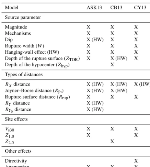
Model ASK13 CB13 CY13
Source parameter
Magnitude X X X
Mechanisms X X X
Dip X (HW) X X
Rupture width (W) X X X
Hanging-wall effect (HW) X X X
Depth of the rupture surface (ZTOR) X X (HW) X
Depth of the hypocenter (Zhyp) X Types of distances
RXdistance X (HW) X (HW) X (HW)
Joyner–Boore distance (Rjb) X (HW) X (HW)
Rupture surface distance (Rrup) X X X
RYdistance X (HW)
RY0distance X (HW)
Site effects
Vs30 X X X
Z1.0 X X
Z2.5 X
Other effects
Directivity X
Attenuation X X X
3 Strong movement models
The CB13, ASK13 and CY13 prediction equations (Camp-bell and Bozorgnia, 2013; Abrahamson et al., 2013 and Chiou and Youngs, 2013, respectively) are considered, so that 5 % damping elastic response spectra for surface type geological faults can be obtained. The database of the first three models is the PEER NGA-West2, which contains over 21 000 accelerograms for the three compo-nents of ground motion of earthquakes recorded in dif-ferent parts of the world, with magnitudes ranging be-tween 3.0 and 7.9. From this record wealth, CB13 employed 15 521 records from 322 earthquakes, while ASK13 em-ployed with 15 749 records of 326 earthquakes. Finally, the model of CY13 employed with 12 444 records of 300 earth-quakes. From this grand total, 2587 records were selected from 18 non-California earthquakes.
All three models have very important databases that ac-credited their equations of ground motion. Table 2 shows the variables that each of the models considers. It shows that there is little difference between them, in general, so that the spectral shapes tend to be similar.
The CY13 model considers the effect of directivity, which is very important when the site of interest is very close to the fault, unlike the other two models that do not consider it. Its formulation is based on studies by Spudich and Chiou (2008) and developed by Spudich (2013). In the first study, the IDP directivity factor (isochrone directivity predictor) is
consid-Figure 4.Soil classification in Quito.
ered. Instead, in the second, the direct point parameter (DPP) model is used, but the variables are expressed incrementally, for example1DPPand1ZTOR, which are also calculated
in-crementally in the CY13 model.
In addition, the CB13 considers the depth of the hypocen-ter (ZHYP) as a paramehypocen-ter in dehypocen-termining the spectral accel-eration, which is ignored in the other models. To check any difference, it is important to consider some strong movement models for the determination of the spectra (for case studies) or ground motion attenuation equations (for seismic hazard studies).
4 Soil classification in Quito
It is important to emphasize that the spectra shape changes according to the type of soil, as can be observed later in Fig. 6. Therefore, a brief explanation of the type of soils in Quito is presented in the following paragraphs. In Fig. 4, the five zones of the Metropolitan District of Quito are pre-sented: south, south-central, central, north-central and north. For each zone it is necessary to determine the response spec-tra associated with blind reverse fault segments. For example, the Puengasí fault starts in the south and reaches the center of the city. Its rupture length, associated with a earthquake of magnitude 6.4, is 22 km (Table 1), so this fault is the source of the highest spectral accelerations in the following areas: north-central, central, south-central and south.
At the north of the city, the fault segment associated with the highest spectral accelerations is Ilumbisí–La Bota (ILB), where an earthquake of 6.2 maximum magnitude is expected (Alvarado et al., 2014). The other faults that exist in the north do not generate spectra with larger ordinates due to being furthest from the city.
They identified three types of soils called S1, S2 and S3 (Aguiar, 2003): (1) in the soil profile S1, the speed of the shear wave isVs30≥750 m s−1, and the periods of soil
vibra-tion are less than 0.2 s; (2) in the soil profile S2, the periods of soil vibration are between 0.2 and 0.6 s and (3) in the soil profile S3 the periods are greater than 0.6 s.
In the NEC-15 norm, there are six types of soil: (1) the soil profile A corresponds to competent rock with Vs30>1500 m s−1; (2) the soil profile B corresponds to
a mean stiffness rock with 760 m s−1< Vs30<1500 m s−1;
(3) the soil profile C has 360 m s−1< Vs30<760 m s−1; (4) in
the soil profile D, the speed of the shear waveVs30is between
180 and 360 m s−1; (5) in soil profile E, the speed is less than 180 m s−1and (6) the soil profile F is a very low resistance soil which requires the presence of a specialist in soils or geotechnical engineer to make an assessment.
To get a better idea of Quito soil types, a seismic refraction study was done in the Metropolitan Park, in a place where there is a rocky outcrop about 30 m high; see Fig. 5. It was found thatVs30=466.27 m s−1, so it is a soil type C (Castillo,
2014). In Quito there is definitely no soil type A, but there are soil types B–D, as shown in Fig. 4.
5 New spectra
The new spectra were estimated at equidistant points (100 m) of a regular mesh and for the three soil types B–D. In turn, this regular mesh was divided into five areas considered in the Metropolitan District of Quito. In each area, and for each type of soil, spectra was obtained at each point of the mesh, using the three ground motion prediction equations indicated above, and finally, an average spectrum was obtained from these spectra.
In the northern area of Quito, an earthquake of magni-tude 6.2, related to the fault segment Ilumbisí La Bota, gener-ates the largest spectral accelerations since it is closer to this area. In the first row of Fig. 6, these spectra are indicated for confidence levels of 50 and 84 %, and for soils B–D. Fault segments Puengasí, Carcelén-El Inca, Bellavista–Catequilla and Tangahuilla generate smaller amplitude spectra for this area.
In the last four rows of Figs. 7 and 8 the spectra for the north-central, central, south-central, and southern zones of Quito are presented for an earthquake of magnitude 6.4 on the fault segment of Puengasí. The other fault segments gen-erate lower spectral ordinates.
6 Recurrence periods
The return period is the time between the occurrence of two events at the same seismic source. Therefore, it is a concept that helps to estimate the expected time of occurrence of an earthquake of a given magnitude.
Figure 5.Rocky soil in Quito,Vs30=466.27 m s−1. Metropolitan Park.
To estimate the recurrence interval associated with differ-ent magnitudes within each segmdiffer-ent, the seismic potdiffer-ential of the fault should be modeled by the moment rate. This pa-rameter (moment rate) estimates the annual accumulation of energy in each segment of the fault and will be used to relate the slip rate to the assigned recurrence model.
6.1 Estimation of the seismic moment rate (M˙0) in each fault segment
From the size of the fault plane of each segment (Table 1), the slip rate of the segment (3.0–4.0 mm yr−1 by Alvarado et al., 2014), and with the conservative assumption that all the plane fault is accumulating energy evenly, the moment rateM˙0can be related to the above parameters according to
expression of Brune (1968), Eq. (3).
˙
M0=µ· ˙u·A, (3)
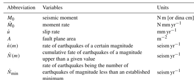
whereµis the shear modulus (103N m−2)isu˙ the slip rate andAis the fault plane area (Table 1). A Supplement with variables and units is included.
6.2 Seismicity rate estimation using the modified recurrence model GR andM0˙
Recurrence models define the seismic potential failure relat-ing the frequency and size of earthquakes occurrrelat-ing in a par-ticular source in a given time. The parameters used to define the potential seismic quakes are the number of earthquakes of a certain magnituden(m)˙ (the inverse of the period of re-currence in a given time unit), or the cumulative rate of earth-quakes of a magnitude higher than a given valueN (m)˙ , and the proportion of large vs. small earthquakes [borβ].
Figure 6.Spectra for the northern zone of Quito.
Figure 7.Spectra for north-central and central zones of Quito.
by Gutenberg and Richter (1944) (GR) and modified by Cosentino et al. (1977) is the most widely used for charac-terizing the source. The Gutenberg–Richter-modified model (Eq. 4) provides a relationship between the cumulative rate of different magnitudesN (m)˙ , the rate of earthquakes being the number of earthquakes of magnitude less than an estab-lished minimum (N˙min), generated at a certain time and in a
particular area.
˙
N (m)= ˙Nmin·
exp(−β(m))−exp(−β (M max))
exp(−β (Mmin))−exp(−β (Mmax))
(4) From the seismic moment rate, a relationship can be estab-lished between this parameter and a recurrence model type GR through the expression of Anderson (1979), Eq. (5).
˙ M0=
Mmax
Z
Mmin
˙
n(m)·M0(m)dm, (5)
whereM0(m)is the seismic moment generated in an
earth-quake of magnitudem.
Moreover, Anderson and Luco (1983) propose relation-ships between the cumulative seismic moment rate M˙0
and three models of recurrence: truncated model, GR-modified model and the recurrence model proposed by Main and Burton (1981).
In this paper, the model GR-modified is used, with Eq. (6), where the cumulative rate of earthquakes of magnitude min-imumN˙min is dependent the on moment rate among other
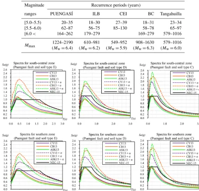
Table 3.Recurrence periods, Gutenberg–Richter-modified model.
Magnitude Recurrence periods (years)
ranges PUENGASÍ ILB CEI BC Tangahuilla
[5.0–5.5) 20–35 18–30 27–39 18–31 23–34
[5.5–6.0) 62–87 56–75 85–130 58–78 65–97 [6.0< 164–262 179–279 169–279 579–1016
Mmax 1224–2190 610–981 549–952 908–1630 579–1016 (Mw=6.4) (Mw=6.2) (Mw=5.9) (Mw=6.3) (Mw=6.0)
Figure 8.Spectra for south-central and south zones of Quito.
˙
Nmin=
˙
M0 d−β
(exp(−β (Mmin))−exp(−β (Mmax)))
β
exp(−β (Mmax)) M0(Mmax)−exp(−β (Mmin)) M0(Mmin)
, (6) where N˙min is the cumulative rate of earthquakes of
mag-nitude greater than or equal toMmin,β is a parameter that
defines the proportion of earthquakes as a function of their magnitude and will be set to 1.84–2.76 (Rivas-Medina et al., 2014b), Mmax and Mmin are the maximum and
mini-mum magnitudes of truncation, M0(Mmax)and M0(Mmin)
are the seismic moments (co-seismic) that would be released in these possible maximum and minimum magnitude earth-quakes, respectively, obtained from the expression of Hanks and Kanamori (1979) andd=1.5·ln(10).
This expression allows the rate of seismic activity of the fault to be deduced. The calculated values are truncated at a maximum and minimum depending on the rate of seismic moment of the fault.
In Fig. 9, the earthquake cumulative rate is presented for different magnitudes, and for each of the segments of the re-verse faults in Quito. From this figure, Table 3 shows the recurrence periods for different magnitude ranges.
As elastic response spectra for maximum magnitudes in each fault segment was obtained, it is interesting to observe the last row of Table 3. For the Puengasí fault, an earth-quake of magnitude 6.4 is expected in a time interval be-tween 1224 and 2190 years; for the Ilumbisí–La Bota fault, an earthquake of magnitude 6.2 is expected between 610 and 981 years.
Figure 9. Earthquake cumulative rate for different magnitudes ˙
N (m)(Rivas-Medina et al., 2014b).
Moreover, the date on which an earthquake with a magni-tude greater than 6.0 associated with the Puengasí or Ilumbisí – La Bota faults occurred is not known, so that compliance with the period of recurrence in these failures can be in a few or many years. The truth is that more than four centuries have passed without a strong earthquake and so the likelihood of a severe earthquake in these two fault segments increases.
7 Commentary and conclusions
Quito is very close to five active segments of reverse faults called, from south to north, Puengasí, Ilumbisí–La Bota, Carcelen–El Inca, Bellavista–Catequilla and Tanhaguilla.
In this paper, monitoring spectra for the horizontal move-ment of the soil were computed, for the five areas of the city, south, south-central, central, north and north central, accord-ing to the classification of soils of the NEC-15.
These spectra were obtained using the models of Abra-hamson et al. (2013), Campbell and Bozorgnia (2013) and Chiou and Youngs (2013) and the maximum magnitude that could be generated in each segment of the blind faults was taken into account. Spectra for the 50 and 84 % confidence levels are also found and the latter have spectral ordinates higher than those found with the NEC-15, so it is important that new construction projects are built in Quito, considering the spectra found in this paper.
Moreover, the recurrence periods were estimated for the maximum magnitude expected in each segment, with which the control spectra recurrence were found, and are between 549 and 2190 years.
Finally, we recommend that the structures should be de-signed for two denominated spectra: design spectra, similar to those stipulated in the NEC-15, and maximum spectra, which were studied in this work with a confidence of 84 %.
The random uncertainty of movement is accounted for through the standard deviation associated with each ground motion prediction equation (the spectra results for 50 and 84 % confidence levels) and the epistemological uncertainty is calculated using the three equations used.
The data on the blind fault system in Quito have been ob-tained in the last 20 years. There are still many uncertainties, not only in this data but in the method and its results. How-ever, there is no time to lose alerting people about the seis-mic danger in Quito. The structural designer must be aware of this fact by means of spectra that use the latest available information.
8 Data availability
Appendix A: Variables and units used to estimate the recurrence periods
Table A1.Variables and units.
Abbreviation Variables Units
M0 seismic moment N m[or dina cm] ˙
M0 moment rate N mm yr−1
˙
u slip rate mm yr−1
A fault plane area m−2
˙
n(m) rate of earthquakes of a certain magnitude seism yr−1 ˙
N (m) cumulative fate of earthquakes of a magnitude seism yr−1 upper than a given value
˙ Nmin
rate of earthquakes being the number of
seism yr−1 earthquakes of magnitude less than an established
Competing interests. The authors declare that they have no conflict of interest.
Acknowledgements. We thank the National Secretary of Higher Education, Science, Technology and Innovation (SENESCYT) of Ecuador for supporting this research.
Edited by: B. D. Malamud
Reviewed by: F. Moreu and one anonymous referee
References
Abrahamson, N. A., Silva, W. J., and Kamai, R.: Update of the AS08 Ground-Motion Prediction Equations Based on the NGA-West2 Data Set, PEER – Pacific Earthquake Engineering Re-search Center Headquarters, University of California, Berkeley, 2013.
Aguiar, R.: Microzonificación Sísmica de Quito, 1st Edn., IPGH, Ecuador, p. 212, 2003.
Aguiar, R., Rivas, A., Benito, M., Gaspar, J., Trujillo, S., Arcinie-gas, S., Villalba, P., and Parra, H.: Aceleraciones registradas y calculadas del sismo del 12 de agosto de 2014 en Quito, Revista Ciencia, 16, 139–153, 2014.
Alvarado, A., Audin, L., Nocquet, J. M., Lagreulet, S., Segovia, M., Font, Y., Lamarque, G., Yepes, H., Mothes, P., Rolandone, F., Jar-rin, P., and Quidelleur, X.: Active tectonics in Quito, Ecuador, as-sessed by geomorphological studies, GPS data, and crustal seis-micity, Tectonics, 33, 67–83, doi:10.1002/2012tc003224, 2014. Anderson, J.: Estimating the seismicity from geological structure
for seismic-risk studies, B. Seismol. Soc. Am., 69, 135–158, doi:10.1016/0148-9062(79)90309-7, 1979.
Anderson, J. G. and Luco, J. E.: Consequences of slip rate constants on earthquake occurrence relations, B. Seismol. Soc. Am., 73, 471–496, 1983.
Bath, M.: A note on recurrence relations for earthquakes, Tectono-physics, 51, 23–30, doi:10.1016/0040-1951(78)90047-1, 1978. Beauval, C., Yepes, H., Bakun, W., Egred, J., Alvarado, A., and
Sin-gaucho, J.: Locations and magnitudes of historical earthquakes in the Sierra of Ecuador (1587–1996), Geophys. J. Int., 181, 1613– 1633, doi:10.1111/j.1365-246x.2010.04569.x, 2010.
Brune, J. N.: Seismic moment, seismicity, and rate of slip along major fault zones, J. Geophys. Res., 73, 777–784, doi:10.1029/jb073i002p00777, 1968.
Campbell, K. W. and Bozorgnia, Y.: NGA-West2 Campbell-Bozorgnia Ground Motion Model for the Horizontal Com-ponents of PGA, PGV, and 5 %-Damped Elastic Pseudo-Acceleration Response Spectra for Periods Ranging from 0.01 to 10 s, PEER – Pacific Earthquake Engineering Research Center Headquarters, University of California, Berkeley, 2013. Castillo, D.: Espectros de diseño para Quito considerando factores
de cercanía asociados a fallas ciegas, Tesis de grado, Universidad de Fuerzas Armadas, ESPE, Quito, Ecuador, p. 160, 2014. CEC – de la Construcción: Capítulo 1: Peligro sísmico, espectros
de diseño y requisitos de cálculo para diseño sismo resistente, XIII Jornadas Nacionales de Ingeniería Estructural, Universidad Católica, Quito, 325–350, 2000.
Chinnery, M. A. and North, R. G.: The frequency of very large earthquakes, Science, 190, 1197–1198, doi:10.1126/science.190.4220.1197, 1975.
Chiou, B. S. J. and Youngs, R. R.: Update of the Chiou and Youngs NGA Ground Motion Model for Average Horizontal Component of Peak Ground Motion and Response Spectra, PEER – Pacific Earthquake Engineering Research Center Headquarters, Univer-sity of California, Berkeley, 2013.
Cosentino, P., Ficarra, V., and Luzio, D.: Truncated Exponential Frequency Magnitude Relationship in Earthquake Statistics, B. Seismol. Soc. Am., 67, 1615–1623, 1977.
Crouse, C. B. and McGuire, J. W.: Site response studies for purpose of revising NEHRP seismic provisions, Earthq. Spectra, 12, 407– 439, doi:10.1193/1.1585891, 1996.
De la Construcción, N. E.: Peligro Sísmico/Diseño Sismo Re-sistente, Código: NEC-SE-DS, Quito, Ecuador, 2015.
Elwood, K: Performance of concrete buildings in the 22 Febru-ary 2011 Christchurch earthquake and implications for Canadian codes, Can. J. Civ. Eng., 40, 759–776, doi:10.1139/cjce-2011-0564, 2013.
Field, E. H. and SCEC Phase III Working Group: Accounting for site effects in probabilistic seismic hazard analyses of Southern California: overview of the SCEC Phase III report, B. Seismol. Soc. Am., 90, S1–S31, doi:10.1785/0120000512, 2000. Gaspar-Escribano, J. M., Benito, B., and García-Mayordomo, J.:
Hazard-consistent response spectra in the Region of Murcia (Southeast Spain): comparison to earthquake-resistant provi-sions, Bull. Earthq. Eng., 6, 179–196, doi:10.1007/s10518-007-9051-4, 2008.
Gutenberg, B. and Richter, C. F.: Frequency of earth-quakes in California, B. Seismol. Soc. Am., 34, 185–188, doi:10.1038/156371a0, 1944.
Hanks, T. C. and Kanamori, H.: A moment magnitude scale, J. Geo-phys. Res., 84, 23480–23500, 1979.
Hao, H. and Gaull, B. A.: Estimation of strong seismic ground mo-tion for engineering use in Perth Western Australia, Soil Dynam. Earthq. Eng., 29, 909–924, doi:10.1016/j.soildyn.2008.10.006, 2009.
Leonard, M.: Earthquake fault scaling: Self consistent re-lating of rupture length width, average displacement, and moment release, B. Seismol. Soc. Am., 100, 1971–1988, doi:10.1785/0120090189, 2010.
Main, I. G. and Burton, P. W.: Rates of crustal deformation inferred from seismic moment and Gumbel’s third distribution of extreme magnitude values, Proc. Earthq. Eng., 2, 937–951, 1981. Nunziata, C., Sacco, C. and Panza, G. F.: Modeling of Ground
Mo-tion at Napoli for the 1688 Scenario Earthquake, Pure Appl. Geo-phys., 168, 495–508, doi:10.1007/s00024-010-0113-1, 2011. Rivas-Medina, A., Santoyo, M. A., Luzón, F. Benito, B.,
Gaspar-Escribano, J. M., and García-Jerez, A.: Seismic Haz-ard and Ground Motion Characterization at the Itoiz Dam (Northern Spain), Pure Appl. Geophys., 169, 1519–1537, doi:10.1007/s00024-011-0405-0, 2011.
Rivas-Medina, A., Martínez-Cuevas, S., Quirós, L. E. Gaspar-Escribano, J. M., and Staller, A.: Models for reproducing the damage scenario of the Lorca earthquake, Bull. Earthq. Eng, 12, 2075–2093, doi:10.1007/s10518-014-9593-1, 2014a.
máx-ima para el control de las estructuras en el rango elástico ante un sismo asociado a las fallas inversas de Quito, Revista Interna-cional de Ingeniería de Estructuras, 19, 201–217, 2014b. Spudich, P.: The Spudich and Chiou NGA-West2 directivity model,
in: chap. 5 in Pacific Earthquake Engineering, PEER – Pacific Earthquake Engineering Research Center Headquarters, Univer-sity of California, Berkeley, 2013.
Spudich, P. and Chiou, B. S.: Directivity in NGA earthquake ground motions: analysis using isochrone theory, Earthq. Spectra, 24, 279–298, doi:10.1193/1.2928225, 2008.
Trenkamp, R., Kellogg, J. N., Freymueller, J. T., and Mora, H. P.: Wide plate margin deformation, southern Central America and northwestern South America, CASA GPS observations, J. S. Am. Earth Sci., 15, 157–171, doi:10.1016/s0895-9811(02)00018-4, 2002.
Valverde, J., Fernández, J., Jiménez, E., Vaca, T., and Alarcón, F.: Microzonificación sísmica de los suelos del Distrito Metropoli-tano de la Ciudad de Quito, Escuela Politécnica Nacional del Ecuador, Quito, 2002.