Paper 13-2009-1

UDC: 556.532:519.87

A Procedure for State Updating of SWAT-Based Distributed Hydrological

Model for Operational Runoff Forecasting

D. Divac1*_{, N. Milivojević}2_{, N. Grujović}3_{, B. Stojanović}4_{, Z. Simić}5

Institute for Development of Water Resources “Jaroslav Černi”, 80 Jaroslava Černog St., 11226

Beli Potok, Serbia; e-mail: 1_{[email protected],} 2_{[email protected],}

5_{[email protected]}

3_{Faculty of Mechanical Engineering, University of Kragujevac, 6 Sestre Janjić St., 34000}

Kragujevac; e-mail: [email protected]

4_{Faculty of Science, University of Kragujevac, 12 Radoja Domanovića St., 34000 Kragujevac,}

Serbia; e-mail: [email protected] *Corresponding author

Abstract

The foundation of operational management of river flows (regarding water resources exploitation, hydropower potential use, flood management, etc.) is accurate and reliable runoff forecast. The systems for operational management support are based on hydrological/hydrodynamic simulation model that uses data on up-to-date states of catchment and prognostic values of model forcing (e.g. precipitation) for prediction of water levels and flows in streams and reservoirs. The best estimate of model forcing (temperature, quantity and distribution of precipitation, etc.) derived from ground measurements and remote sensing is crucial for success of simulation model use. This paper discusses the application of “data assimilation” procedure for updating simulation model state variables using mainly model forcing data. The term itself relates to a set of mathematical methods designed for use of measured data and differences between simulated and measured values in up-to-date model state estimation and forecast of future states in physical systems. These methods allow for better parameterization, structural and sensitivity analysis of the model, as well as design of more efficient observation networks and improving forecasts and quantitative measures of their reliability. The paper presents an approach to operational use of SWAT-based rainfall/runoff hydrological model, using an algorithm for rainfall distribution estimation based on data from few automated weather stations. The implementation of presented algorithm in “Drina” hydro-information system confirms the sensitivity of the simulation model to forcing data, and provides improvements of the runoff forecasting, bringing the mentioned model into operational use.

1. Introduction

A precise and reliable forecast of water inflowinto a storage represents the basis for efficient

operational water resource management, including warning and flood protection, storage

exploitation, and regulation of the rivers. The core of contemporary systems for operational

forecast of water inflowis the hydrologic/hydrodynamic simulation model, which uses the data

on the up-to-date state of a catchment and the forecast of input data (precipitation and the like)

in order to calculate water levels in storages and discharges along the rivers. The accurate

forecast of the distribution of precipitation on a catchment is a pre-condition for a successful

application of a hydrologic model. The temporal-spatial resolution that is needed for the

forecast of precipitation varies depending on the application, basin, type of precipitation, and the model to be used.

A great effort has been recently put into the application of different observed hydro-meteorological and other data for the analysis of hydrologic processes (Walker et al. 2001; Reichle et al. 2002; Crosson et al. 2002; MacKay et al. 2003; Sun et al 2004; Ni-Meister et al.

2006; Dong et al. 2007). The data on a certain parameterthat are in this way entered into the

models can also be independent, for instance, microwave images of soli humidityor “in situ”

humidity measurements (Ceballos et al. 2005). It is also possible to improve the forecasted

values of a certain quantity by the means of the assimilation of diverse data, like it was

presented by Aubert et al. (2003) in the case of inflowforecastand the assimilation of observed

discharges,and “in situ” observed values of soil humidity.

Even more complicated is the application of observed data on inflow forecast for the

purpose of hydropower plant management. This management can be strategic, i.e., periodically performed, or operational, which is a daily activity. Strategic planning includes the comprehension of strategic goals, which are the optimum ones for the integrated system that the facility belongs to, as well as for the hydropower facility in question. Operational planning represents the realization of strategic plans, which leads, on the basis of the forecasted inflows and the distribution of demands, to the physical management of a plant. In addition to all this, it is necessary to take into account that a hydropower system can consists of several power plants that operate in a cascade, or are sometimes coupled with a reversible power plant. In such cases, the complexity of a problem increases because the operation of the power plants is closely coupled and an additional set of operational limitations of exploitation has to be applied. In the paper Divac et al (2009), the role of a hydro-information system in strategic and operational planning is presented. In this paper the assimilation techniques were implemented for the needs of inflow forecasting and those techniques will be further discussed below.

Almost all hydrologic models used for the operational forecast of inflow into storages are deterministic. That means that the input data (e.g., precipitation, temperature etc.) is processed and on that basis the output data (for example, discharges, snowmelt etc.) is calculated. The measurements of output variables represent the redundant information because the model does

not allow the ambiguityof the output data. For this reason, it is necessary to take into account

that operational models cannot offer perfectly precise values of output variables.

In order to use all the data in the best possible way, it is necessary to quantify the reliability

of each information source, which includes measured outputs,estimated inputs and variable of

the model state. If it is possible to quantify all the data sources in this way, it is then also

possible to apply the methods of the state estimation theory, which determine the combinations of data resources that offer the best estimations of the previous, current and future states of a hydrologic system.

The state estimation theory takes into account the total distribution of probabilities of

“the best estimation” of the previous, current and future states. The application of the Kalman filter (Gelb 1974) on hydrologic modeling offers wide possibilities in the field of operative hydrology, although it brings along certain problems that have to be solved.

Another approach, which in the first place takes into account input data, is the application of the “data assimilation”. The name itself denotes a set of mathematical methods, which allow

for the use of the observed data and the deviationof the calculated values from the measured

ones in the process of estimation of the up-to-date model and the forecast of the future states of physical systems. The examples of the application of this approach can be found in oceanography, geophysics, and meteorology (Bennett 1992; Berliner 2003; Daley 1991), where on the basis of satellite and ground observations more accurate forecasts can be achieved. In hydrology is the application of this method of importance in the process of linking of the model

of the underground water balance with the observed precipitation (Walker et al. 2002). These

methods allow for better model parameterization,analysis of model structure and its sensitivity

to disturbances, development of more efficient observance networks and improved forecasts together with quantified measures of their reliability.

This paper presents the approach to the operational use of a hydrologic model based on the

SWAT calculations of rainfall/runoff (Simić et. al., 2009), by the means of the algorithm for the

estimation of rainfall distribution on acatchmenton the basis of a smaller number of automated

precipitation stations. The results obtained by the application of the mentioned algorithm and model confirm the sensitivity of the model based on SWAT to the distribution of precipitation on the catchment and demonstrate improvements in the case of the application of the algorithm for the precipitation forecast on a catchment.

2. Principles of data adjustment in hydrologic models

Generally speaking, there are two possible approaches in relation to the application of hydrologic models to water resources management (which means at the same time to hydropower facilities); the one is long-term planning (i.e., strategic planning) and the other one is short-term planning, which is used for the acquisition of operational forecasts of inflows into

storages, i.e. for the real-time management support (operational planning). The first approach

relies on the use of the historical seriesfor the calibration of the parameters of a model; this is

performed in order to employ the model for long-term forecasts of the behavior of the system, or for the analysis of solutions with several variants for the development of hydro-technical facilities on a catchment. A model that is calibrated using a longer period of time can produce more accurate evaluations of different scenarios and improve the quality of hydrologic studies, what significantly contributes to the quality of the strategic planning of water resources management and consequently to the development of the suitable legal regulations. In the

second case, the up-to-date observationsof the state of the model and the inputs into the system,

along with the current forecasts from the hydro-meteorological service, are entered into a distributed hydrologic model, in order to simulate the balance of surface and underground waters on a catchment. The estimation of the state of the model is performed in this way in

order to improve the forecastof the inflow into storage to meet the needs of the operational

planning of the exploitation of water resources and hydropower objects.

ambiguities. In order to meet the needs of the short-term forecast of the state of a catchment it is necessary to implement certain feedback mechanisms, which have an influence on a reduction of the difference between the results of the model and the observations, which results in a more reliable forecast of the catchment runoff. Such mechanisms are called data assimilation or

updating of the model state,and they represent the core of any operational system that relies on

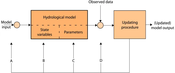
hydrologic models (Madsen et al., 2002). During a longer period of time dedicated to research, four basic approaches have been implemented in practice. The ways in which these approaches exert influence on a hydrologic model itself are presented in Figure 1. The common feature of all four approaches is that the model updating procedure relies on the noticed differences

between the calculated and observed quantities,as well as the fact that the resulting variables of

the model are the functions of input values, the computational state of the model and its parameters.

Fig. 1. The possible approaches to assimilationofdata into hydrological simulation models

Approach A: The correction of input data represents one of the first applied updating methods of the computational state of the model. The principles of the method itself are relatively simple

to comprehend, because the values of these variables, measured in the nature, must be applied

with great caution when used in hydrologic models (precipitation, temperature, etc). Taking into

account the possible deviations of the measured values from the real oneswithin a catchment, it

is practically always justified to correct them in order to achieve the up-to-date computational

state. The actual correction of input values affects the computational model state, what allows

for its convergence towards the state of the real system. This method also certain disadvantages, too. First of all, taking into account a possible large number of input variables, the determination of their correction factors could a too difficult optimization problem. Besides, the model itself is in this case considered perfectly correct, what, of course, can never be true. For these reasons, the application of this method requires the models that are as accurate and as detailed as possible and that have, in the same time, been calibrated as well as possible.

Approach B: The direct updating of the model state variablesis performed on the basis of the

established differences between the calculated and the observed values (of water levels and

dischargesat control points, observed soil humidity, water content in the computationalelement

of the model etc.). It is possible to apply several different procedures that are based on statistical methods. The simplest method is based on the direct replacement of the computational values by the observed values. Naturally, very often this be not correct from the computational point of

view, taking into account that this procedure violates the laws that the model is based upon,

because the distributions of the variableobtained by the application of the interpolation method

model during the simulation. More advanced methods are based on the application of the

Kalman filter, which allows for the determination of the state valuesin a way that is close to

physically-based models. In this case the statistical evaluation of temporal-spatial error

correlations within the model is used (Brummelhuis, 1996). It is currently a common practice to make use of advanced implementations of Kalman filter, which allow for the determination of the estimation of the distribution of precipitation (Todini, 2001) and the estimation of the states of hydrologic models (Grijsen et al., 1992).

Approach C: The updating of the parameters of the model is performed with the goal of

minimization of the difference between the computational and the observed values, what is

achieved by the means of the change of the parameters of the model depending on the identified

error in output quantities. It can be considered that the repeated change in parameters is

performed because of the neglecting of certain phenomena during the period of the first calibration (Young, 2003). This method is most often applied to models based on data, while its application to deterministic physically-based models is extremely rare. In such cases, the

parameters of the surface runoff coefficient,flow resistance etc. can be changed so that one can

speak about the constant periodical recalibration of the model,although it is not expected from

the parameters that are determined on the basis of the analysis of the catchmentareato differ to

a large extent from their initial values. Generally speaking, it cannot be expected that the

physical features of a basin can greatly change during such short periods of time.

Approach D: The updating of output quantities is based on the statistical structure of the

model; in this case, instead of the correction of input valuesor the parameters of the model, the

error estimationis performed, on the basis of the structure of the model and the current results.

The value of the forecasted variableis corrected on the basis of the forecastederrorin order to

achieve the final forecastedvalue.For such procedures, auto-aggressive methods are used, such

as the ARMA (auto-regressive moving average) of the model. These procedures are simple and

they do not demand the extreme engagement of processor resources. The examples of this

procedure applied on hydrology can be found in the papers Refsgaard (1997) and Madsen et al. (2002).

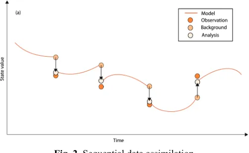
Fig. 2. Sequential data assimilation

The second classification of the methods of data assimilation can be performed according

to the method that is operationally used for the determination of the up-to-datecomputational

state of the model;in this case, there are two possibilities: the sequential data assimilation and

Sequential data assimilation (presented in Figure 2) assumes that the calculation should be performed using only upon the last observed values, as soon as they become available. This approach leads to the appearance of a discontinuity in the moments observed before and after a certain up-to-date state. This approach is suitable in cases when the system behavior is dominantly determined by the external boundary conditions.

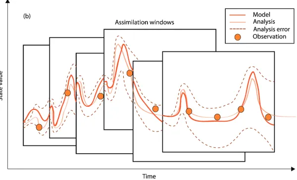
Fig. 3. Variationalor indirect data assimilation

Variational or indirect data assimilation (in Figure 3) assumes the use of all observed data since the beginning of the application of the model until the present moment and in order to determine the solutions that globally offer the best congruence with the measurements. This approach appears very often in meteorology, where the current states of a model dominantly depend on the initial state of the simulation.

3. Basic principles of the proposed methodology of determination of the up-to-date state of hydrologic quantities within a catchment

When simulation models are applied for the forecast of inflowsintostorages, certain deviations

of the forecasted from the actual values can appear. These deviations appear due to the errors in the states of the model, which are the consequence of the imperfection of the model, the usage of parameters that are not the optimum ones and of low-quality input data. For this reason is the

procedure of data assimilation often applied in the systems for the forecast of inflow, in order to

allow for the update of the states of the system and their harmonization with the observed values.

The typical forecast of inflows into storages is performed on the basis of the data from

multiple sources. The calculation begins from a historical moment in which the values of the

state of a catchment are known (or supposed) and these values become the initialconditionsfor

In the calculation it is possible to use the data from various sources, with the adequate

weighting. The calculations are performed periodically, usually on a daily basis. Taking into

account the fact that the calculation period depends on the features and implementation of the model, it is important to determine how far it is reasonable “to go” into the past or the future.

Namely, the initialconditions of the calculation are often the results of the previous calculation,

so that they usually do not correspond to the current state of the system. It is therefore necessary to perform a calculation, at least for the period that has been analyzed in the previous calculations. On the other hand, the future period should not be too long, since the reliability of the input data (the forecasted values in this case) decreases in proportion to the length of the period for which the forecast is performed.

There are no general recommendation or guidelines regarding the choice of the length of the period of the calculation, but would be convenient that this length should encompass all the major phenomena in the system, for instance, the formation of flood waves due to precipitation

(for this to happen it is necessary for a certain hydrographto reach its maximum value due to

propagation of the wave) etc. If the occurrence of the successive disturbancesis expected (the

two waves that can be superimposed), their total duration has to be taken into account, too.

In large basins there are almost always storages that regulate the flow of waterand that can

be used for different purposes such as electricity generation, irrigation, water supply or flood

prevention. In the case of electricity generation, besides flow regulation there are also

independent processes related to the electricity generation and transmission system, which additionally complicate storage management. The operational management of such facilities relies on the reliable inflow forecasts, i.e. on operational hydrologic models. One of the main conditions for the implementation of operational hydrologic models is the existence of the

methodology for the determination of the up-to-datecomputationalstate.

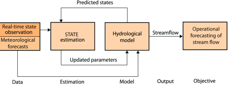
Fig. 4. The procedure of the formation of the operational forecast of the inflowfrom a catchment according to the proposed methodology

computational state of the model is the initial conditionfor the calculation of forecasted inflows

and it is obtained for the forecasted values of system input variables. The scheme of this

procedure is presented in Figure 4.

In practice, the optimization module periodically runs the calculations for the defined previous period until the state of the model that conforms to the known, observed data, is

reached. After that, upon the basis of the forecasted inputs, the forecast of the catchmentrunoff

is created. In the Figure 5 is presented the general principle of the formation of the operational forecast.

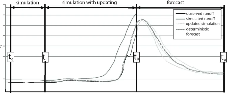
Fig. 5. The principle of the formation of the operational inflow forecast

The goal of the formation of the operational forecast of catchment runoff is the

determination of the runoff in the future period of interest, which can be one or more days long, depending on the available meteorological forecasts and the requested forecast accuracy. This goal can be achieved in a few subsequent steps.

During the period between t-2 and t-1 the simulation is performed on the basis of the known

model state and the measured input data. Taking into account the known state and the input data of the model, during this period there is a satisfactory congruence between the calculated and observed data.

After the moment t-1 the procedure of updating of the computational model state begins.

During the period from t-1 to t0 the correction of the available input data is performed in order to

achieve the computational state of the model that results in the computational runoff that is close to the observed one. During this period, the iterative process of the application of the optimization module is performed, with the goal of determination of the optimum values, which are used for the correction in order to minimize the deviations of the calculated runoff from the

measured catchment runoff. If this optimization problem is successfully solved, then at the

moment t0 an up-to-date computational model state becomes available.

Upon the basis of the updated computational model state at the moment t0 the process of

runoff forecast begins. During the forecast period from t0 to tp the calculation of the runoff is

performed on the basis of the meteorological forecast. From the meteorological forecast model

the values are taken, which are then assignedas the inputfor the hydrologic model. In this way,

relying on the up-to-date state at the moment t0 the forecasted catchmentrunoffis formed. The

main role of the up-to-date model state at the moment t0 is to prevent the possible deviations of

this reason is the procedure of updating of the computational model state irreplaceable in any operational prognostic model.

3.1. Model of transformation of rainfall into runoff

The models of transformation of rainfall into runoff, or, generally speaking, the models of

catchment areas, can be very simple, as, for example, the conceptual models (Burnash, 1995;

Havno, 1995). By the means of well-calibrated conceptual models, it is possible, on the basis of

measured meteorological values, to determine catchmentrunoff(which is usually observed as

discharge on the exit profile of the catchment) with a sufficient accuracy. Even greater accuracy

can be achieved by the means of distributed hydrologic models. The distributed models take into account also the spatial distribution of model parameters, what means that they require a larger amount of input data. In order to meet the need for a large amount of data in hydrological and hydro-informational modeling and simulation, the use of geo-informational system and related technologies increases. This approach has actually become a standard. Some of the most popular distributed hydrologic models are TOPMODEL (Beven, 1997), MIKE SHE model (Refsgaard and Storm, 1995) and SWAT model (Arnold et al., 1998).

A detailed overview of the development of the SWAT model is given in the paper Simić et

al. (2009). The development of this model has been progressing in accordance with the capacity for collecting real physical data, and it involves so far a large number of different physical processes that are simulated within a basin and which are relevant for the simulation of water

flowwithin a basin.

The developed SWAT model is based on the calculation of the state within each Hydrologic Response Unit. The Hydrologic Response Unit (HRU) is a concentrated land area within a catchment, which has homogenous soil composition and the same regime of land use.

The calculations provide for the preservation of water balanceon the level of a HRU and also of

the catchment itself. This model is based on five linear reservoirs: the land cover reservoir, accumulation and snowmelt reservoir, surface reservoir, underground reservoir, and surface

runoff reservoir. Water balancehas to be satisfied for each reservoir. The relationships between

the reservoirs are of such a nature that they use the physically possible water flow paths,which

are flow, seepage, percolation, evapotranspiration, and underground flow.

The successful calibration of the model is presented in the paper Milivojević et al.

(2009ab), where the issues of the parameter choice, sensitivity analysis, and criteria for the evaluation of the calibration quality were also discussed. Taking into account the importance of the calibration of the model for the operational purposes, the indicators of the quality of input

data were discussed in detail (GIS data, hydro-meteorological data etc.). The inaccuracies in the

historical measurements of temperatures and precipitation were demonstrated, as well as the

fact that the segments of time seriesare often filled-inwith a certain level of reliability. Taking

into account the above-mentioned, the sensitivity analysis was also performed. This analysis defines the main guidelines for the choice of the parameters that should be estimated.

3.2. Input data for the model of transformation of rainfall into runoff

According to this methodology, during the period of the updating of the model state, input time series are generally corrected upon the basis of additional observations that indicate the deviation of calculated values from the real states of the catchment. Hence, it is necessary to comprehend the sources of such data, its reliability and how it affects the model state.

 Input data – values of the quantities that do not belong to the states of the system; it can consist of measured and forecasted values,

 Parameters – charateristics of the process that is being modeled, and

 Observations of the state of the model – values of quantities that describe certain

some state of the model and are used for the control of the model and forecasting. The following table presents the values that are relevant for the used hydrologic model, as well as the categories and data sources. The category determines the mode of use of certain data in the simulation model and the source represents the mode that is used in order to obtain certain data.

Data category Data source

Data Input _{data of the model} Parameter Observation of _{the state surveying} Field Numerical _model Other

Precipitation • • •

Evaporation • • •

Air temperature • • •

LAI •

Vegetation type • •

Soil characteristics • •

Hydrographic

network • •

Surface waters •

Runoff • •

Table 1. The values relevant for the used hydrologic model

The greatest influence on the state of the model has precipitation, which can be determined in various ways, depending on the measurements that are present at a certain catchment. The

configuration of the system for the observation of precipitation affects to a large extent the

mode of the use of measurements, in order to meet the needs of the model. Besides precipitation, mean daily temperatures also represent a very important parameter, which can be used in somewhat easier way as model input, considering that its spatial distribution is much more evenly balanced spatial than in the case of precipitation. The conditions under which is the discussed being used and the suggested methodology for the determination of the up-to-date calculated state applied, determine one of the following two possibilities: a) only point measurements from a smaller number of automated stations within the basin are available, or b) some numerical meteorological models are available, which offer the distribution and intensity of precipitation in the form of two-dimensional fields.

In the first case, the data on precipitation are entered into the model in the form of points,

which represent the meteorological stations where the meteorological quantitiesare measured.

methods of interpolation; by this method a transition is made from the level of information in a

pointto the spatial data regarding the influence of the particular meteorological stations on the

resulting spatial distribution. In this approach to the assignment of precipitation data and in order to make corrections to the input data one can speak of the choice of the interpolation method, correction of the parameters of the interpolation method and of the correction of the time series itself that are recorded on the measurement sites.

In the second case, each point in a catchment can by the means of its coordinates copy the

precipitation data from a 2D precipitation field, which is the result of the numerical model.

Taking into account direct copying, there is no more need for interpolation. However, it is only

possible to correct the precipitation fielditself, with the minimum possible disturbance of the

distribution itself. This can be achieved by the means of the introduction of a correction plane,

which linearly adds/subtractsthe precipitation defined by the precipitation field.

4. Creation of input data of a hydrologic model on the basis of measurements on meteorological stations

Each forecast system requires the optimum state of the system at the moment t0 (the moment at

which the forecast begins). For this reason, it is crucial for each forecast system to re-calculate the state in the immediate past before the beginning of forecasting. The correction of the input data is the primary goal in improvement of the system state, what should lead to the better

matching between the calculated values of discharges and water levels with the measured

values.

The precipitation data, which is available for assignment, is specified in the form of values

on individual meteorological stations. Considering the fact that it is known where these stations are located in real space, it is possible to perform the spatial interpolation by the means of one of the mathematical methods, which leads to a transition from the level of one-dimensional data to spatial two-dimensional data.

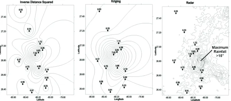
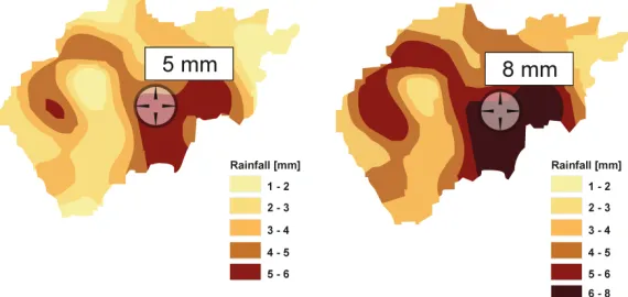
Fig. 6. The comparison of the different interpretations of precipitation

perform the correction of the time series recorded on the measurement sites.The justification of the particular selection can be demonstrated by Figure 6; this figure presents the distributions of precipitation, which are obtained by the means of two different interpolation methods, along with the representation of the actual distribution of precipitation. It can be noticed that none of the methods describes this natural phenomenon in a satisfactory way.

4.1. Interpolation methods

The methods of interpolation of the spatial distribution of precipitation are of great importance for the GIS (Geographical Information System) solutions, which is the reason why it is possible to find a large number of implemented methods in this field of study. Of course, some of the methods have been developed for particular cases, what limits their application to a smaller number of problems they can solve. However, there are numerous methods of the general type that can be applied to most cases.

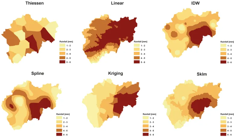
Fig. 7. The resulting distribution of precipitation depending on the selected interpolation method

Figure 7 demonstrates the resulting distribution of precipitation depending on the selected interpolation method. The comparison of the presented results indicates huge differences in the distribution due to the application of different mathematical principles. In further text an overview of the most commonly used methods will be presented.

4.1.1. Thiessen’s polygons

Thiessen’s polygons, also known as Voronoy’s diagrams, are the polygons whose boundaries

determine the planes that are closer to the center of gravity of its own polygon than to the

centersofgravityof other polygons. In the case of the precipitation stationsthis means that the

Let (

Z

precipitation Z on the location u, where no measurements are performed, can be obtained by the

means of the following expression:

u i

Z Z hui   h iuj j (1)

where:

 Zu are interpolated values at the point u,

 Zi is the measured value on the ith measurement location,

 huiis the distance between the location without measurement u and the location with

measurement i and

 hujis the distance between the location without measurement u and the location with

measurement j.

4.1.2. Spline method

This method makes use of the technique of the minimization of the curvature for the

interpolation of the plane in space, which 1) passes precisely through the points with

measurements,and 2) possesses the minimum curvature.For the interpolation of the plane, the

following formula is used:

1

( ) n

u u ui ui i

Z T





 



where:

 Zu is the interpolated value,

 n is the number of measurement locations,

 λuiare the coefficients obtained by solving of a system of linear equations and

 hui is the distance of the location u without measurements from the location i with

measurements.

The trend function Tu and the generative function R(hui) are determined by the spline

parameters and the detailed description of this method is presented in the papers Franke (1982) and Mitas and Mitasova (1988).

4.1.3. IDW method

The IDW (Inverse Distance Weighted) method of interpolation is explicitly based on the presumption that phenomena which are spatially closer to each other are more similar to each

other than to some other spatially distant phenomenon. This method assigns larger weight

coefficients to the points with measurements, which are closer to the interpolation point; the

result of this is that the influence of a certain point, in which the measurements have been

performed, on the final valueis inversely proportional to the distance of that point from the

point of interpolation.This is defined by the following expression:

1

1

1 n

u n ui i i ui i

Z  Z

   





where:

 Zu is the interpolated value,

 n is the total number of points with measurements near to the interpolation point,

which are used in the process of interpolation,

 Zi is the value in the ith point with measurements,

 hui is the distance between the interpolation point u and the point with measurements i

and

 λui is the weight coefficient of the ith point with measurements.

4.1.4. Kriging method

Kriging is the name of the geostatic method, which offers the best linear unbiased estimator. It is called unbiased because the mean value of the error estimation equals zero and the adjective

“the best” is used because its application leads to the minimization of the variance of errors.

The unknown amount of precipitation Z in the interpolation point u is estimated as a linear

combination of the values of the adjacent pointswith measurements as:

1

n u ui i

i

Z









where:

 Zu is the interpolated value,

 Zi is the value in the ith point with measurements and

 λ is the weight coefficient of the ith _{point with measurements.}

Instead of the inverse proportionality of the weight coefficients to a certain degree of

distance of the interpolated point from the points with measurements, the standard Kriging

method is based on the spatial correlation structure of data for determination of weight

coefficients. For determination of weight coefficients two presumptions are used: 1) provision

of the unbiased nature ofthe estimator(s) as:





0; 2

u u

E Z Z  (5)

and 2) the minimization of the variance of estimation as:





u u

Var Z Z (6)

where Z_u*denotes the measured value.

The Kriging method makes use of a half-variogram for the determination of weight

coefficients that surround the interpolation points, what is usually achieved by solving a system of linear equations, generally known as “the standard Kriging system” (Goovaerts, 2000):

 

 

 

1

n

uj ij ui j

h u h

   



 



1 1 n uj j   

where:

 μ(u) is the Lagrange parameter that limits the weight coefficient,

 hui is the difference of the point without measurement u from the point with

measurement i and

 hij is the distance of the points in which the measurements were performed i and j.

The half-variogram γ(h) is calculated as:

 

_{  }



2

N h

i i h i

h Z Z

N h





where:

 h is the distance between two points,

 N(h) is the number of pairs of points separated by the directionh and

 zi – zi+h is the difference of the value in the point i and the value in another point

separated from it by the directionh.

A more detailed description of the Kriging method is presented in the paper Isaaks and Srivastava (1989).

4.1.5. Linear regression

Due to the orographic effect, the precipitation increases with an increase in altitude. This is

proven by the means of different examples by Hevesi et al. (1992) and Goovaerts (2000). The altitude can be taken into account by the distribution of precipitation in a simple manner that is by the regressive linear function:

0 1

( )

u u u

Z  f y a  a y (10)

where:

 yu is the altitude of the interpolation point u and

 a0and a1are the regression coefficients calibratedfor the known set of measurements.

4.1.6. The simple Kriging with variable local means

The simple Kriging with variable local means, abbreviated SKlm) was presented by Goovaerts

(2000) as the simplified Kriging where the known stationary mean value of the observed

quantity is replaced by the variable mean valuemu, which is derivedfrom secondary data as:

 

1

n u u ui i

i

Z m





 



where Ri Zimi.

Local mean values can be obtained by the means of the linear regressive function. In that

case, the estimated precipitation in the interpolation point u can be expressed as:

 

 

1

n u u ui i

i

Z f y





where the weight coefficients λuiare obtained by solving the standard Kiriging system:

 

 

1

n

uj R ji R ui j

C h C h









where

C h

( )

(Goovaerts, 2000). The other varibles have already been explained. For more details on the SKlm method see Goovaerts (1997).

4.2. Automated interpolation of data on precipitation for meteorological stations

As it has already been mentioned, in order to correct input data, what is performed with the

purpose to achieve the up-to-date state, the interpolation of the point measurements from the

available meteorological stations is performed. Taking into account the fact that the goal here is the estimation of the model state, which would represent the state that is closest to the one of the real system, the automated interpolation of input data related to precipitation is performed, which as a result has the spatial distribution of precipitation in a basin. Each hydrologic

computational unit has the corresponding coordinates, so that its precipitation will be

determined by the means of the following formula:









p x y F x y k p k p k p (14)

where:

 p (x,y) is the interpolated precipitation in the point with the coordinates x and y,

 0

j

p is the observed precipitation on the meteorological station j,

 Fi is the selected interpolation function (Thiessen's polygons, spline method, IDW,

Kriging etc.) and

 k is the correction factor for the meteorological station j.

From the presented formula it is obvious that it is possible to choose an interpolation

method Fi, perform the correction of the parameters of the selected interpolation method (if it

has any), and to the corresponding extent, by the means of factors kj, perform the correction of

the time series, which are recorded at the measurement sites themselves. The determination of the optimum choice of the interpolation method, as well as of the optimum correction factors that would produce the computational state of the model closest to the real state of the system, represents a specific optimization problem.

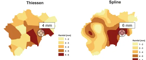
Previous figure presents the influence of the change of the selected interpolation function on the value of the interpolated precipitation in the point (x,y). It is obvious that in certain sections of a basin significant differences in the interpolated values can appear. In the Figure 8, the change in the precipitation for the fixed hydrological calculation unit is presented and it can be observed that the difference in values amounts to 150% appeared when instead of Thiessen’s polygons the spline method of interpolation has been applied.

Fig. 9. The change in the values of the interpolated precipitation due to the application of correction factors

Besides, the measurements obtained from the automated meteorological stations can exhibit a certain local character and they can contain measurement errors due to wind etc. Hence, it is justified to perform the correction of the measured values themselves. In the Figure 9 the influence of the change in the corrective factors on the values of the interpolated precipitation in the point (x,y) is demonstrated.

5. Creation of input data of a hydrologic model on the basis of forecasted data

The formation of input data of a hydrologic model on the basis of forecasted data can be implemented in the case of meteorological numerical models that continuously produce the forecast of the distribution of the precipitation on the observed catchments. The numerical models of the meteorological forecast make use of mathematical formulations of the processes in the atmosphere in order to make weather forecasts. Such models provide meteorological information on the future state of the atmosphere. For example, The Republic Hydro-Meteorological Service of Serbia makes use of two models for its operational work. The first one is the Eta model, which twice a day creates the forecast for the next 120 hours and covers the territory of Europe, the Eastern Atlantic and the Northern Africa. The second model is the

WRF-NMM model, which is of mezo scale of the latest generation, with a complex physical

model and advanced numerical methods. The horizontal resolution of the model is circa 10 km.

The simulation is performed twice a day, with boundary conditionsfor the next 72 hours and it

covers the Balkans and the Adriatic Sea. Such models present the forecasted values in the form of a network of points, the number of which depends on the discretization of the model.

The main goal of this procedure, just like the previous one, is the determination of the

up-to-date state of the computational model upon the real state of the catchment, in order to

minimize the difference between the calculated and the observed runoff. Taking into account

necessary to define the mode of the correction of the whole network, while attempting to disturb the numerically obtained distribution as little as possible. For this reason, the concept of a

correction planeis introduced, which performs the linear correction of the spatial precipitation

obtained by the means of a numerical model. It can be stated that the correction is performed according to the following expression:

, , ,

,

o i j i j i j i j

p k p

k   i  j

 

     (15)

where:

 pi,jis the corrected precipitation at the point of the network which belongs to row i and

column j,

 p°i,j is the calculated precipitation in the point of the network which belongs to row i

and column j,

 ki,jis the correction for the point of the network which belongs to row i and column j

and

 α, β, γ are the parameters of the correction plane.

The main goal of this procedure is to find the parameters of the correction plane that correct precipitation in such way that during the period of updating the model produces the calculation runoff, which to a minimum extent deviates from the observed and recorded runoff. As one of

the extreme cases can be marked the solution α = 1, β = 0. γ = 0. what means that the

precipitation offered by the forecast model is further used without any correction.

Figure 10 presents the case of the correction of precipitation with a correction plane

described by the following parameters α = -1.2, β = 0.1, γ = -0.01. In this way, the precipitation

in the North-Eastern part of the catchment is reduced and the precipitation in the rest of the catchment is proportionally increased.

The problem of determination of the parameters of a correction plane that correct precipitation in such a way that during the period of the updating the model produces the calculation runoff that to a minimum extent deviates from the observed and recorded one, represents an optimization problem which can be solved by the means of one of the optimization methods. Taking into account a relatively small number of the parameters of the model, it is possible to apply one of the direct methods of minimization without limitations. Direct methods require only the calculation of the objective function, without the need for the search for the derivative of the function. These methods are also known as the methods of the zero rank because they perform the search on the basis of the zero derivative of the goal function. Generally speaking, these methods are inferior in comparison with the gradient methods, but considering the fact that in this particular case a small number of management variables are used, they can be successfully applied.

All methods of optimization without limitations are basically of the iterative nature, where

the process begins by the application of the initial trial solution and in each step it is

approaching the optimum. It is important to notice that all optimization methods are based on

the defining of the initial solution X1and that they differ only in the method that they use in

order to move to the next solution Xi+1, and the procedures for verificationwhether a particular

solution is the optimum one. It can therefore be concluded that the main disadvantage of these methods is the possibility of convergence towards the local minimum, which brings into the foreground the quality of determination of the initial solution. For this reason, in this paper it is proposed to apply the unification with the previous procedure of the correction of

meteorological measurements which are obtained from the network of the measurement

stations, as well as the application of genetic algorithms in order to solve both optimization

problems.

6. Applied optimization algorithms

As a platform for the solving of the demonstrated optimization problems, genetic algorithms are proposed, which are able to determine the position of the global optimum in the space with multiple local extremes (in the so-called multi-modal space). Classic deterministic methods always move towards the local minimum or maximum, whereby it can also be global in some cases, but that cannot be determined from the obtained results. Stochastic methods, which include genetic algorithms, do not depend on the initial solution and they can due to their search

procedureslocate the global optimum of the observed function with a certain probability.

Generally speaking, the evolution algorithms significantly differ from the traditional

methods of searchingand optimization. The main differences are the following:

 Evolution algorithms simultaneously search for the results in multiple points and not

only in individual points;

 Evolution algorithms requireno information on function derivatives, or on any other

analytical calculation and the direction of the search is only influenced by the objective

functionand the levels of fitness;

 Evolution algorithmsuse probability lawsand not deterministic laws;

 These algorithms are mostly easier to realize than the traditional methods of searching

and optimization and

 Evolution algorithmscan offer several possible solutions for a certain problem and the

user can in the end make his choice. This is important for problems which are not completely defined, so they can have multiple solutions (multi-parameter optimization etc).

A genetic algorithm consists of the initialization and the evolution (which consists of selection, crossover and mutation). During the initialization the primary population of solutions

is generated. The initial population is usually generated by the random choiceof solutions from

the domain of the acceptable solutions; however, it is more convenient to start from the values of the last known state of the system. The process that follows this stage is then repeated until one of the criteria of convergence is satisfied. That process consists of the action of the genetic

operatorsof selection, crossoverand mutation upon the population. During selection the inferior

solutions “die out” and the superior ones “survive”, so that in the next step the superior

solutions “cross over” and “mate”, what leads to the transfer of the features of the “parents” to

their “offspring”. The mutation changes the features of the solution by a random change of genes. By such a procedure the quality of population increases from one generation to another and the advantageous ratio of diversity to convergence is maintained; this allows for avoidance of the situation where the algorithm stops after finding a local optimum. For the concretization of the algorithm, it is necessary to determine for each of the problems the following: the method of defining the solutions in a form that is suitable for genetic algorithms, as well as the specific

objectivefunction,i.e., the method for verificationofthe validity of the solution.

6.1. Definition of solutions in the form suitable for genetic algorithms

The procedure of the transformation of a real solution into a form that is suitable for genetic algorithms is one of the most important procedures in the implementation of genetic algorithms, because the efficiency of the algorithm greatly depends on the form of the solution in question. Taking into account that the procedure is strongly related to the nature of the problem, each implementation requires a separate analysis of the possible definitions of the problem.

All the data that create one individual (i.e., one solution) are written into one chromosome. For example, let the problem be one-dimensional, i.e., let the the global optimum of the

objective functionwith one variable f(x) in the known search area x

 

this case one individual, i.e., one chromosome, represents one solution_x*_,x*_

 

(in this case it is one real number) can be stored within one chromosome in different ways.

This procedure mostly often consists of the recording of a real numberx into a sequence of bits,

which create one chromosome, i.e., into a binary code. In this way a real number x is

represented with accuracy that depends on the number of the used bitsn. These discrete values

that can in one way or another appear as a part of the solution that can be estimated by the objective function. By the means of this procedure, it is possible to transform a large number of

problems into binary form.

In the first case, the solution consists of the ordinal number of the selected interpolation

method Fi (which belongs to the set of available methods) and the needed number of

correction factors

k

meteorological stations. Hence, the solution consists of N1 numbers, which are binary coded.

In the case of an optimization problem, which relates to the formation of input data of a hydrologic model upon the basis of forecasted data, the solution consists of the values of the parameters of the correction plane. Thus, the solution consists of 3 real numbers respectively,

which correspond to the parameters , ,   , which are binary coded.

6.2. Defining of the fitness of the solution

The fitness of the solution indicates its quality. When defining the fitness, the objective

function, whose extremes (the minimum or the maximum) are searched for, is of crucial

importance. In the case of both proposed methods, the objectivefunctionis the same and taking

into account the fact that it defines the total deviation of the calculated from the observed

hydrographs, the goal is its minimization. In a general case, on a complex basin (which consists of many sub-basins), numerous measurement stations can exist. In the course of calculation of the fitness, it is necessary to use measurements from all of them. Considering the fact that the

fitness is defined by the objectivefunction, which is a real number, when applying its definition

it is necessary to use all the measurements in the normalized form.For this reason, the objective

functionhas the following form:





, ,

1

1

R

o i j i j M j i i Q Q f Q    _             





where:



Q

 o_, i j

Q is the observed dischargeon the station i at the moment j,

 Qi is the mean annual observed dischargeon the station i,

 M is the number of hydrological stations and

 R is the number of the steps of the hydrograph.

Taking into account the fact that the goal here is the minimization of the deviation, it follows that the goal of optimization is exactly the minimization of the defined objective

function.For this reason, the fitness of the solution is defined as the reciprocal value of the





, ,

1

1

1 o _R

o i j i j M

j i i F

Q Q

Q







 _ 

 

 



 

 

 





(17)

The determination of the fitness of the proposed solution is reduced to its decoding, performing of simulation for specified values and calculation of the objective function on the basis of the obtained computational discharges.

7. Application of the proposed methodology within a hydro-information system with an example

7.1. Importance of determination of the up-to-date state of the simulation model in a hydro-information system

Within the structure of the hydro-information system presented in the paper Milivojević et al.

(2009a), the calculations that are related to hydrologic and exploitation processes are based on the simulation model and on-line services that make use of it. In order to meet the needs of the intake forecast, the simulation module, which is managed by the optimization module, is used; this particularly holds true for the part of the simulation module that performs rainfall/runoff

calculations (Simić et al. 2009).

In order to use the model operationally, it is necessary to develop the service for the calculation of the up-to-date state and the forecast of catchment runoffs. This HIS-service is composed of the simulation and the optimization module. Its primary purpose is the assimilation of the data related to the states of the system, as well as bringing the up-to-date state of the model closer to the real state of the system. This is achieved by the periodical automated performing of calculations, where the optimization model takes care of the goal that the results of the calculations of the simulation model should be as similar as possible to the observed states of the system during a certain period. The resulting values of the model states are stored in the database and are considered the updated states of the model for all calculations until the expiring of the given period. After the expiring of the given period, the procedure is repeated and the newly obtained state is considered the new up-to-date state. The availability of the up-to-date model state allows for the operational use of the model for the forecasting of the

inflow and managementin real-time.

7.2. An example of determining of the up-to-date state of the simulation model within the “Drina” hydro-information system

The application of the proposed methodology and the corresponding simulation and optimization modules on this catchment, as well as the details on the catchment are presented in the paper Divac et al. (2009). In the same paper is also defined the structure of the hydro-information system, with the specific features of its application to the River Drina basin.

For the demonstration of the process of the formation of the operational forecast of the

inflow from basin, the watercourse of River Lim has been selected, with the associated

sub-basins. There are no dams and storages on this watercourse and it is therefore suitable for the analysis of the efficiency of the procedure for updating of the model state and its influence on the quality of forecasting of the catchment runoff. For the control of the output results of the model, the measurement data on the hydrologic station “Prijepolje” are used; for this station there is the up-to-date discharge curve and the automated measurement of the water level is also performed on that station.

The configuration of the simulation model is presented in Figure 11, which is taken from the simulation program the “Drina” HIS.

For the application of the model the typical spring-period is chosen, with clearly pronounced precipitation and the characteristic catchment runoffs. Figure 13 presents the precipitation during the given, for the precipitation stations “Plav”, “Andrijevica” and

“Goševo”. These stations are located in the area of the leading, upstream sub-catchments.

Fig. 13. The precipitation during the analyzed period in the area of the leading,

upstream sub-catchments

In the Figure 14, the precipitation in the areas of the downstream sub-catchments, which are much closer to the hydrologic station “Prijepolje”, is presented. The precipitation on the stations “Berane” and “Bijelo Polje” is presented. The data from the other relevant stations is also entered into the model, but it is not presented here because of the limited available space (only the data from the most representative stations is shown here).

Fig. 14. The precipitation during the analyzed period on the precipitation stations “Berane” and “Bijelo Polje”

Fig. 15. The mean daily temperatures during the analyzed period

7.3. Results of the application of the up-to-date state of the simulation model

The example of the application of the service for the calculation of the up-to-date state consists of the periodical generating of the weekly forecast of the catchment runoff. Every run of the weekly forecast presumes the existence of the up-to-date computational state of the model at the beginning of the forecast. In Figure 14 the time cross-sections in which the up-to-date state was formed are presented by red dots in the diagram. The blue line represents the historical measurements of runoffs from the subject hydrologic measurement station.

Fig. 16. The comparison of the measured, simulated, and forecasted (without updating) values of the model outputs

the weekly forecast it is possible to notice somewhat higher deviations in relation to the observed runoffs. Such a trend can be expected, because during the periods with greater precipitation the meteorological model is not capable of producing the forecasts for a period that is several days long with a great accuracy. Taking into account that after seven days it is possible to observe the deviation of the calculated state of the model from the observed values, the new updating of the model is performed.

The red dashed line represents the forecast obtained upon the basis of the meteorological forecast, but without the updating of the computational model state. It is evident that, due to the insufficient matching of the calculated state and the state of the system, such a forecast in the course of time progressively deviates from the observed runoffs. Namely, due to the imperfection of the model and the incompleteness and unreliability of the input data, in calculations which are performed without periodical updating of the model state the errors accumulate in time, so that such calculations cannot offer a reliable forecast of the catchment runoff.

In the analyzed example it is demonstrated that the application of the techniques of data assimilation for the periodical updating of the model state significantly increases the usability of the existing simulation model, and that, consequently, the resulting forecasts can be used for the purposes of operational management of river watercourses and storages.

8. Conclusions

Taking into account the growing availability of measurements, significant efforts are being made in order to apply the diverse hydro-meteorological and other observed data to the field of hydrology. The assimilation of various data can help the improvement of the forecasted values of catchment runoffs (with the application of in situ observed values). However, even more complicated is the application of the observed data for the forecasting of inflows used in order to meet the needs of the operational management of hydropower plants. In the process of

solving these issues, the necessary accuracy of forecasting of inflowscomes becomes evident,

because hydropower systems are mostly relatively complex and the operation of the facilities that these systems consist of is often coupled and often predominantly influenced by the inflow from the catchment.

Mathematical methods which allow for the use of the observed data and the deviations of the calculated from the measured values in the process of the estimation of the up-to-date model and the forecast of the future states of physical systems have proven their suitability for the application within the operative hydrologic models. In this paper, two cases which occur in practice, and which are related to the updating of the computational state of the model were analyzed. The first case is the one when only a small number of measurements from the automated meteorological stations are available. The other case is related to the systems in which it is possible to provide the precipitation on the catchment in the form of numerical meteorological models. Both solutions rely on the correction of the available precipitation data, whereby, in the first case mathematical interpolation of the measurements in a point is performed.

genetic algorithms, together with the defining of the objective function that mathematically defines the quality of the solution.

It is necessary to notice that the data assimilation itself does not necessarily lead to the improvement of the operational use of hydrologic models. In order to make the assimilation possible, it is necessary to have available an accurate and well-calibrated model, as well as the indicators of the quality of data collected in real-time. Besides, it is necessary to find the balance between the complexity of the model, data resolution and required accuracy, in relation to the time available for the solving of such complex optimization problems.

In the future it is necessary to consider the most efficient ways inclusion of these methods into the existing hydro-information systems, while creating at the same time strong links to data validation services, other simulation models, forecasting systems etc. It is also necessary, taking into account the development of observance systems and hydro-information systems themselves, to envisage an extensible platform that can perform the assimilation of other types of measurements, too.

References

Arnold JG, Srinivasan R, Muttiah RS, Williams JR (1998), Large area hydrologic modeling and assessment – Part 1: model development. Journal of the American Water Resources Association, 1998. pp. 73–89. No. 34.

Aubert D, Loumange C, Oudin L, Le Hegarat-Mascale S (2003), Assimilation of soil moisture into hydrological models: the sequential method. Canadian Journal of Remote Sensing 29: 711–717.

Bennett AF (1992), Inverse Methods in physical oceanography. Cambridge University Press, New York. 370 p.

Berliner LM (2003), Physical-statistical modeling in geophysics. Journal of Geophysical Research – Atmospheres 108(D24): 8776.

Beven KJ (1997), Distributed Hydrological Modelling: Applications of the TOPMODEL Concept. John Wiley & Sons, 1997.

Brummelhuis PGJ (1996), Kalman filtering in real-time control systems. In Proceedings of the 2nd Hydroinformatics conference, M¨uller A. (Ed.), Balkema, Rotterdam.

Burnash RJC (1995), The NWS river forecast system – catchment modeling. In Computer Models of Watershed Hydrology. Water Resources Publications, 1995. pp. 311–366. Ceballos A, Scipal K, Wagner W, Martinez-Fernandez J (2005), Validation of ERS

scatterometer-derived soil moisture data in the central part of the Duero Basin, Spain. Hydrological Processes 19: 1549–1566.

Crosson WL, Laymon CA, Inguva R, Schamschula MP (2002), Assimilating remote sensing data in a surface flux – soil moisture model. Hydrological Processes 16: 1645–1662. Daley R (1991), Atmospheric data analysis. Cambridge University Press, New York. 474 p.

Divac D, Grujović N, Milivojević N, Stojanović Z, Simić Z (2009), Hydro-Information Systems

and Management of Hydropower Resources in Serbia, Journal of the Serbian Society for

Computational Mechanics, Vol. 3, No. 1

Dong J, Walker JP, Houser PR, Sun C (2007), Scanning multichannel microwave radiometer snow water equivalent assimilation. Journal of Geophysical Research 112: D07108. Franke R (1982), Smooth Interpolation of Scattered Data by Local Thin Plate Splines. Comp. &

Maths. with Appls. Vol. 8. No. 4. pp. 237–281. Great Britain.

Gelb A (1974), Applied Optimal Estimation (Cambridge, MA: MIT Press).