Paper 10-2017-1

(DOI: 10.24874/jsscm.2017.11.01.10)

Incremental Finite Element Formulation for Large Strains Based on the

Nodal Force Increments

M. Kojic1,2,3*_{, V. Simic}1_{, M. Milosevic}1,4

1 _{Bioengineering Research and Development Center BioIRC Kragujevac, Prvoslava Stojanovica}

6, 3400 Kragujevac, Serbia e-mail: [email protected]

e-mail: [email protected]

2 _{Houston Methodist Research Institute, The Department of Nanomedicine, 6670 Bertner Ave.,}

R7 117, Houston, TX 77030, USA e-mail: [email protected]

3 _{Serbian Academy of Sciences and Arts, Knez Mihailova 35, 11000 Belgrade, Serbia} 4Belgrade Metropolitan University, Tadeuša Košć_{uška 63, 11000 Belgrade, Serbia} *corresponding author

Abstract

In this paper, we introduce an incremental formulation for large strains which is based on the nodal forces increments. It uses the linear strain increments at the current configuration as the fundamental strain measure, and consequently the stress increments which produce the nodal force increments. It does not assume any total strain and stress calculation according to total values of (large) displacements. It rather employs summation of internal finite element nodal forces during the incremental-iterative computational procedures. Solutions according to this new formulation are compared with a standard updated Lagrangian formulation, with the Green- Lagrangian strains evaluated using the total displacement derivatives with respect to the current reference configurations. The presented incremental-force based formulation can be considered as a generalization of the use of logarithmic strains.

Keywords: Large strains, finite elements, force-based incremental formulation, linear stain increments

1. Introduction

In general, there are two types of nonlinearities in finite element (FE) analyses: geometrical and material (K. J. Bathe 1996, Kojic et al. 2005). The geometrical nonlinearities come from large displacements which lead to significant changes in the body (structure) position in space and/or significant changes of shape. On the other hand, material nonlinearities are due to nonlinear stress-strain relationships (constitutive laws).

98

There are different strain measures introduced in theoretical considerations and in the FE applications. They, in general, can be defined with respect to different reference configurations, and therefore can have different values for a given displacement field. The results, or the material model response, depend, of course, on the adopted strain measure. This is particularly pronounced in cases of large strains. Motivated by this fact, we introduced here an incremental nodal force-based FE solution procedure (FI) which uses the (small) strain increments only, with respect to the current configuration, as it the case of small strain definition. We consider that this is a natural consequence of the definition of strains.

A summary of definitions of strain measures is given in the next section, and further in Section 3 we formulate the new incremental FE procedure. Numerical examples in Section 5 illustrate the application of the Green-Lagrangian strains and our FI procedure, and differences in the material deformation when using these two formulations.

2. Strain measures

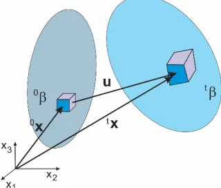
Consider a material body which moves in space accompanied by material deformation. We consider two configurations: (1) initial 0ẞ, assumed to be undeformed, and current (deformed) tẞ, according to Fig. 1. The initial position of a material point is defined by the

Fig. 1. Initial and current (deformed) configurations of a material body

vector 0_{x (coordinates} 0_x

i) and at the current configuration by tx (coordinates txi). The displacement vector u is:

0

t

= −

u x x (1)

The first part of the formulation of a mechanical model represents kinematics of material deformation. The fundamental kinematic quantity which describes the material deformation is deformation gradient:

0 0 0 ; 0 0 0

t t

i i

ij ij

j j

x u

X

x δ x

∂ ∂

∂ ∂

= = + = = +

∂ ∂ ∂ ∂

x u

X I

x x (2)

0 0 0 ; 0 0 0 0 0 0 0

t t

j

T T m m i m m

ij ij

i j j i i j

u

x x u u u

C

x x δ x x x x

∂

∂ ∂ ∂ ∂ ∂

= = = + + +

∂ ∂ ∂ ∂ ∂ ∂

C X X (3)

The Green-Lagrangian strain is defined as:

(

)

0 0 0 0 0 0 0 0 0

1 1 1

; =

2 2 2

j

i m m

ij ij ij

j i i j

u

u u u

e

x x x x

ε  ∂ ∂  ∂ ∂ η

= − _ + _+ = +

∂ ∂ ∂ ∂

 

ε C I (64)

where

0 0 0

1 2 j i ij j i u u e x x  ∂ ∂  = _ + _ ∂ ∂

  (5)

and

0 0 0

1 2 m m ij i j u u x x η = ∂ ∂

∂ ∂ (6)

are linear and nonlinear Green-Lagrangian strain components. Note that the strains are defined with respect to the initial configuration as the reference configuration. In our further analysis we will use the Green-Lagrangian strain with respect to the current configuration, as:

1 1

=

2 2

j

i m m

t ij t t t t t ij t ij

j i i j

u

u u u

e

x x x x

ε _ ∂ + ∂ _+ ∂ ∂ = + η

∂ ∂ ∂ ∂

  (67)

where

1 2

j i

t ij t t

j i u u e x x  ∂ ∂  = _ + _ ∂ ∂

  (8)

and

1 2

m m t ij t t

i j

u u

x x

η = ∂ ∂

∂ ∂ (9)

The strain increments are:

t

ε

η

∆ =∆ +∆ (10)

The second part of the mechanical model description is related to stresses within material. We will use the Cauchy stress definition as force per current area, as:

t t

d F d A

σ = (11)

where dt_{F is the elementary surface force acting on the elementary material surface d}t_A. Therefore, the stress tensor σijcorresponds to the deformed configuration. The stress tensor can be calculated using a material law which specifies relations between stresses and strains, and represents the material property. In general, we can write a relation:

( )

ij f ij

σ = ε (12)

(4)

100

For linear elastic material, this relation is:

;

ij Cijkm km i Cij j

σ = ε σ = ε (13)

where, in usual FE formulations, the one-index notation for stresses and strains is used (with engineering shear strains), and the constitutive 4th _{order tensor is replaced by the 2}nd _order

constitutive matrix. Also, stresses can be specified using the linear part of strains (K. J. Bathe 1996), as:

i C eij j

σ = (14)

In the FE derivations, it is important to notify that the principle of virtual work is the fundamental principle for all established balance equations. The virtual work per unit material volume, at a material point of the deformed material, is defined as:

ij t ij ij t ij

W e

δ =σ δ ε =σ δ (15)

where the virtual strains are infinitesimally small so that the nonlinear part can be neglected without any restriction on generality.

3. Finite element equations of balance

Here, we derive FE equations of balance of linear momentum neglecting inertial forces, which do not depend on the definition of strains. Equations based on the Green-Lagrangian strains (with respect to the current configuration – UL formulation in (K. J. Bathe 1996)) are derived first, followed by our FI concept of large strain FE models.

3.1 Application of the Green-Lagrangian strains

The virtual strains, using isoparametric FE formulation, can be expressed in the form:

L t ie tBij Uj

δ

δ

where

δ

(16)

BL

is the linear strain-displacement

matrix with derivatives of interpolation functions with respect to the current material coordinates tx_i. Detailed expressions for this matrix are given in standard FE books (K. J. Bathe 1996, Kojic et al. 1998). For example, the first row for a 3D continuum is:

1 2

11 12 13 14 15 16

1 1

, 0, 0; , 0, 0 ....

L L L L L L

t t t t t t t t

N N

B B B B B B

x x

∂ ∂

= = = = = =

∂ ∂ (17)

The virtual work of the nodal forces due to stresses within material is:

int int

T L

j j t ij i j

W F U B U

δ

δ

δ

σ δ

On the other hand, using stress increment representation, we have:

(

)

(

)

L t L t

t ij i i j t ij i ik t kj j j

W B U B C B U U

δ = σ + ∆σ δ = σ + ∆ δ (19)

where the increments of stresses are expressed using the constitutive relation (13). The matrix

displacements. The expressions for the terms _tB_kj follow from (8) and (9), and, for the first row

we have:

3

1 1 2 1 1 1 2

11 11 12 13 14 14

1 1 1 1 1 1 1 1

, , ; , ....

L L

t t t t t t

u

u N u N N u N

B B B B B B

x x x x x x x x

∂

∂ ∂ ∂ ∂ ∂ ∂ ∂

= + = = = +

∂ ∂ ∂ ∂ ∂ ∂ ∂ ∂ (20)

In case of using the constitutive law of the form (14), we replace the matrix tB in (19) by tBL.

The incremental equation for iteration i for a finite element is:

( )i−1∆ ( )i = ext− int( )i−1

K U F F (21)

The stiffness matrix K( )i−1 and the internal force vector are: ( )_{i 1}

(

)

t t V dV − − ₌

∫

K B C B (22)

( )

(

)

inti1 LT i

t V dV − − ₌

∫

F B σ (23)

Note that the solution depends on the right-hand side only, while the number of iterations is conditioned by the tangential property of the stiffness matrix (K. J. Bathe 1996, Kojic et al. 2005). Of course, in case of the constitutive law (14), the matrix tBL replaces tB in (22).

3.2 Incremental solution using nodal force increments at the current configuration, i.e. the FI formulation

Here, we start by the increment of stress:

LT t t

∆ =σ B C U∆ (24)

which relies on the tangent constitutive law,

t t d d = σ C

e (25)

where dte are linear strain increments according to (8).

Next, we write the incremental equation (21) in the form:

( )i−1_∆ ( )i ₌ ext₊t int_{+ ∆} int(i−1)

K U F F F (26)

where

( )_{i 1}

(

)

LT t L

t t V dV − − ₌

∫

K B C B (27)

( )

(

)

inti 1 LT i

t V

dV

− −

∆F =

_∫

Here, tFint is the nodal force vector at the start of time step, and increments are calculated with respect to end of the previous step. The strain increments and the matrix tBL(i-1) are

102

( )

( )

2 i j i i t ij j i u u e x x − − _∂ ∆ ∂ ∆ _ ∆ = +  ∂ ∂   

(29)

In case of dynamic analysis, inertial forces must be added. Using the above relations, we can write Eq. (26) in the form of incremental velocities, as it is done in our PAK-SF FE program (Kojic et al. 2017):

( )1 ( ) int int( 1) ( )1

1 i i ext t i 1 i

t

t t

− − −

 _{+ ∆} _{∆ = + + ∆ − ∆}

_∆  _∆

 M K  U F F F M U (30)

where M is the element mass matrix (Kojic et al. 1998, Kojic et al. 2008). The above computational scheme represents our FI formulation.

Therefore, in practical application, we must save element nodal forces due to material deformation t_Fint _{at the start of time step, and to calculate their increments as described above.}

Stress increments correspond to the (linear) strain increments with respect to the last configuration. On the other hand, in the so-called updated Lagrangian formulations (K. J. Bathe 1996), strains are evaluated from derivatives of the total displacements with respect to the current material coordinates. Differences in our force-based FI and the UL solutions come from the fact that the strain increments, and therefore stress and nodal force increments, are not the same for these two formulations. This can be seen from the strain definitions, namely:

( )

2 2

t t t

t t t

UL _{j j}

i i

ij t t t t t t

j i j i

u u

u u

e

x x x x

+∆ +∆ +∆ +∆ ∂ ∂  ∂ ∂  ∆ = _ + _− _ + _ ∂ ∂ ∂ ∂

    (31)

is not the same as:

( )

(

) (

)

2

t t t t t t

FI i i j j

ij t t t t

j i

u u u u

e x x +∆ +∆ +∆ +∆ ∂ − ∂ −    ∆ = + ∂ ∂     (32)

Of course, for small strains these increments are approximately the same.

The proposed concept can be considered as a generalization of the logarithmic strains, since we have: log ln i i l e l λ ∆

= =

∑

where λ is material element stretch and l is the length. To illustrate differences in the UL and FI formulations, we consider uniaxial deformation of elastic material element of the length ₀with the Young modulus E. Then, according to the UL formulation, we have that the strain and displacement are: 0 / UL UL UL u e E u σ = = +  and 0 / 1 / UL E u E σ σ =

−  (34)

0

ln 1 /

FI

FI i

i

l u

e E

l σ

 

∆

= = _ + _=

 

∑

and

(

)

FI E

u = eσ −  (35)

4. Examples

In order to obtain results where we compare solutions for our force- based (FI) and updated Lagrangian (UL) formulation, we considered first a one element case, with uniaxial and shear loading, and with elastic constant and nonlinear Young’s modulus. Then we implemented our FI formulation to model a circular elastic body (tumor) subjected to volume change due to volumetric strain increasing linearly with time (constant growth rate).

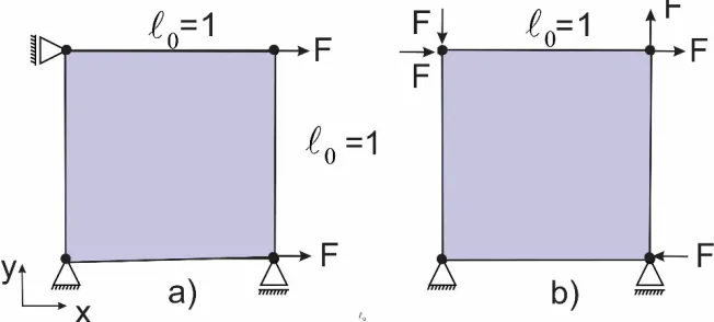
4.1. Plane strain element subjected to uniaxial extension and to shear loading

The 4-node plane strain element with the boundary conditions and loads is shown in Fig. 2.

Fig. 2. One plane strain 2D element loaded by: a) Uniaxial tension and b) Simple shear. Length is in mm and force is in N

The load in Fig. 2a represents uniaxial tension and in Fig. 2b is the so-called pure shear. First, linear- elastic material is used for both uniaxial tension and shearing case, with Young’s modulus – E = 1 [N/mm2], and Poisson’s ratio ν = 0 and ν = 0.499. _{Then, it is assumed a}

nonlinear dependence of the Young modulus on the material stretch.

a) Tension, constant E

104

Fig. 3. Displacement of the free end in terms of stress, UL and FI formulations

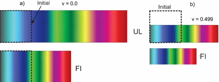
Fig. 4. Displacement field for uniaxial tension for UL and FI formulations, final configurations. a) Case ν = 0 and b) ν = 0.499

b) Shear, constant E

Fig. 5. Shear angle vs nodal force diagrams in case of simple shear for UL and FI formulation for Poisson’s ratio: a) ν =0 and b) ν =0.499

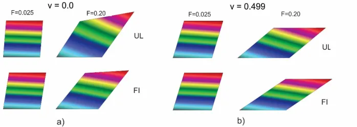
Fig. 6. Displacement field for shear loading for two values of force F and UL and FI formulations. a) ν =0 and b) ν =0.499

c) Uniaxial loading, E depends on stretch

Here we consider the deformation of the unit-size plane strain element subjected to uniaxial loading, in case when Young’s modulus increases nonlinearly with the material stretch. This kind of dependence of Young’s modulus on stretch is present in biological tissue. The dependence E(λ) is shown in Fig. 7.

106

Fig. 7. Dependence of Young’s modulus on stretch

3 2

0 0 0 0

1

t t t T t t t i i i i

λ

=

= =

∑

B X X p p (36)

where ₀t i

λ are principal stretches, and t i

p are the principal directions of the tensor ₀t_{B. In case}

of uniaxial loading, the first principal direction is in the direction of loading.

We here use the FI formulation only, considering it as relevant for large strains. Dependence of the displacement on the axial stress is shown in Fig. 8. The displacement field is analogous to the one shown in Fig. 4. Different character of the relation displacement-stress can be noticed with respect to Fig. 3, since the material becomes stiffer with loading.

Fig. 8. Uniaxial loading, nonlinear E(λ), FI formulation. Dependence of displacement on the stress. a) ν =0 and b) ν =0.499

d) Shear loading, E depends on stretch

As in case of uniaxial loading, there is also difference in character of the angle-force dependence with respect to the case of E=const. (Fig. 5). The shape of the deformed element is similar to those shown in Fig. 6.

Fig. 9. Shear loading, nonlinear E(λ), FI formulation. Dependence of displacement on the stress. a) ν =0 and b) ν =0.499

4.2. Circular body deformation due to volume increase (tumor model with growth rate)

It is known that tumors grow over time. That occurs due to mass generation and a characteristic of growth is the tumor growth rate. The growth rate represents the volume change per unit time and unit volume. We here consider a 2D representation of a circular tumor with isotropic material and with isotopic growth rate. Due to a symmetry we use ¼ of the circle with appropriate boundary condition shown in Fig. 10, with the radius of R=5mm. A linear elastic material is used with Young’s modulus – E = 0.1 [N/mm2], and Poisson’s ratio is ν = 0.499. The

number of nodes for FE model is 317, and the number of plane strain elements is 285. The growth rate is e_V= 50.4 s-1_{. The number of time steps is 25 and step duration is 1s.}

108

Figure 11 gives a radial displacement of the tumor boundary uradial vs Time. The enlargement of

the tumor is almost linear during time.

Fig. 11. Radial displacement of the tumor surface uradial vs. Time, the FI formulation

Fig. 12. Displacement field for growing tumor model, configurations at t=1s and t=25s. Use of the FI formulation

4. Conclusions

(small) strain increments at the current configuration and does not involve any stress or strain summation over the course of material deformation.

Acknowledgements

The authors acknowledge support from Ministry of Education, Science and Technological Development of Serbia, grants OI 174028 and III 41007, and the City of Kragujevac.

References

Bathe KJ (1996). Finite Element Procedures, Prentice Hall, Upper Saddle River, N. J., USA. Kojic M and Bathe KJ (2005). Inelastic Analysis of Solids and Structure, Springer Berlin,

Heidelberg New York.

Kojic M, Slavkovic R, Zivkovic M, Grujovic N (1998). Finite Element Method I, Faculty of Mechanical Engineering (in Serbian), Kragujevac.

Kojic M, Slavkovic R, Zivkovic M, Grujovic N, Filipovic N, Milosevic M, Isailovic V (2017).

PAK-SF Finite Element Program for Linear and Nonlinear Analysis of the Solid-Fluid Interaction, Bioengineering R&D Center, Kragujevac, 2017.