Estimation in Censored Sample Using Linex Loss Function

ISSN (e): 2250-3021, ISSN (p): 2278-8719

Vol. 04, Issue 01 (January. 2014), ||V5|| PP 07-12

Estimation in Censored Sample Using Linex Loss Function

Binod Kumar Singh

University of Petroleum & Energy Studies, Dehradun-248007, India

Abstract: -In life testing experiment, it is common practice to terminate the experiment when certain numbers of items were failed or a stipulated time has elapsed. In order to overcome these situations terminate most of the life tests before all the items fail. Pandey (1977) considered an exponential distribution which is generally used in life testing experiment. Epstein & Sobel (1953) and Bhattacharya & Srivastava (1974) have also considered the censoring procedure in life testing problem. Pandey and Malik (1994) proposed an improve estimator for variancein exponential distribution. In this paper proposes an estimator for variancein case of exponential distribution and studies its properties under Linex loss function.

Keywords: - Linex Loss Function, Censoring, Mean Square Error

I.

INTRODUCTION

In life testing experiment, it is common practice to terminate the experiment when certain numbers of items failed or a stipulated time has elapsed. In order to overcome these situations terminate most of the life tests before all the items fail [Sinha (1980, 1986)]. To avoid this, many life tests are terminated before all the items fail. Let us consider the first n ordered statistics x(1), x(2),……, x(n) in a sample of size (r), in this case the sample is censored on the right which is also called as Type II censoring. Similarly censoring on the left is called Type I censoring. For example, in many biological experiments, r samples from each living things are tested for antibodies after a certain period of time , only „n‟ of these samples contain measurable amounts while remaining (n-r) of the animal develop the antigen at a level too low for measurements. Cohen (1965) and Srivastava (1976) have obtained the likelihood estimates of the parameters in case of continuous distributions such as exponential, normal, log-normal and logistic when samples are progressively censored under the assumption that the parameters of the distribution under consideration might change at each stage of censoring. In such experiments after first stage, the experiment is continued with the remaining surviving items. The idea of removing some items at every stage of censoring stamps from the fact that these items might be required for use somewhere else for related experimentation. Bhattrchaya and Srivastava (1974) have also proposed type I and type II error for censoring process.

Let x1,x2,...,xnbe a random sample of size n from normal distribution with mean θ and variance θ 2

.In some practical situations, prior value of mean and variance are θ0 and θ0

2

respectively. The preliminary testimator for the mean was suggested by Bancroft (1944) as:

If θ0 is the estimate of θ ifH0: 0is accepted, otherwise consider usual estimator

x

or in other words

   



 





otherwise ,

accepted is

: H

if 0 0

0 x

PT

  

 (1.1)

According to mean square error criterion, MSE(₀)E(₀)2 and

n x MSE

2

)

( 

Katti (1962) suggested that _{0 0} 2

2

) ( ) ( )

(  MSE E 

n x

MSE if xR where R is determined by the

testing of hypothesis of  ₀. Also,

 



     

 

   

 

   

 1 1

0 1

n x

where α is the level of significance. Now equation (1.2) can be re-written as

 

 

 _ 

  

 

    

 _{1 0 1} 1

0

n x

n

P (1.3) Here distribution of

x

is known.

Pandey (1977) considered exponential distribution which is generally used in life testing distributions having mean θ and variance θ2

.The improve estimator for θ is

1 0 , ) 1

( 0

1kx k k

P 

The value of k for which risk will be minimum is

n n

k

1 1

1

) (

) (

2 0

2 0

2 2 0

2 0 m in

     

 _

    

 _

  

 

 

 

  

 

which is less than one.

Here the value of k depends on n and

 0 _.If



0 _{=1then k}

min =0 and estimator is0.

The magnitude of relative efficiency will be maximum at



0 _{=1 for smaller level of significance (α) and smaller}

value of n.

Epstein and Sobel (1953) and Bhattacharya and Srivastava (1974) have also discussed censoring procedure in life testing problem and proposed an estimator as

   



 





otherwise ,

accepted is

: H

if _{0 0}

0 1

r PT

cT

  



Since 0

2 

x n

follows chi-square distribution with 2n degree of freedom. Also if

) ( )

( )

2 ( ) 1

( x xr xn

x    and r is the censored data of type II censoring then,

) ( 1 ()

)

( _r

r

i i

r x n r x

T   

 (1.4)

Since



r

nT 2

follows chi-square distribution with 2r degree of freedom i.e.

 

r T V r T E r T V r T

E r r r _r

2 ,

, 4 2 , 2

2 

 

 _ 

                 

If case of two populations with common mean, the unbiased estimator for common mean in exponential distribution is

2 1

2 2 1 1 1

n n

x n x n T

 

 if 22 2

2

1  

  

Pandey and Malik (1994) have considered the improve estimator for θ2 in exponential distribution as

6 ) ( 5 )

( _{1 2} 2 _{1 2}

2 1 2

   

 

n n n

n

y n x n

which is in the form of improve estimator of θ2 in exponential distribution as suggested by Pandey and Singh (1977). Thus ) 3 )( 2 ( 2 2 ' 1    n n x n T

Let us consider displaced exponential distribution having density function



, ,



1







,  ,



0







e x A x A

A x

f (1.5)

Here A is location and  is scale parameter. The maximum likelihood estimators for  and A are and

x

₍₁₎

respectively.

Also



 





1

2nxx

follows chi-square distribution with 2(n-1) degrees of freedom and other researchers have also

considered preliminary estimators/adaptive estimators/ conditional specifications [Han etal (1988), Hogg (1974), Pandey and Singh (1977), Hirano (1973)].

In section 2, proposes an estimator for variance (θ2) in case of exponential distribution as 2 1 2 2 1            r r T T c

Y r r which provide

2 1 21 1 3 2 2 2 1

3 wTr w Tr wTrTr

Y    and studies its properties under Linex loss

function.

II.

ESTIMATION OF VARIANCE IN EXPONENTIAL DISTRIBUTION

UNDER LINEX LOSS FUNCTION

Pandey and Singh (1977) have proposed improve estimator for θ as

                        _  otherwise , 1 1 accepted is : H if 1 0 0 0 r r a T e a   

 (2.1)

Similarly if considered the improve estimator for θ2 as

2 1 2 1           r r T T_{r r}

Pandey and Malik (1994) have also proposed improve estimator for θ2 as

2 1 21 1 3 2 2 2 1

2 wTr w Tr w TrTr

Y    (2.2)

The MSE criterion will provide





4 2 1 3 2 2 2 1 1 1 2 2 2 2 2 2 2 2 1 1 2 3 2 2 2 1 2 3 2 2 1 1 3 1 2 2 1 1 2 1 1 1 1 1 2 1 2 1 ) 1 ( ) 1 ( 2 ) 3 )( 2 )( 1 ( ) 1 ( ) 1 ( ) 2 )( 1 ( 2 ) 1 ( ) 1 ( 2 ) 1 ( ) 1 ( 2 ) 3 )( 2 )( 1 ( ) (                                          r r w r r w r r w r r r r w r r r r w r r r r w w r r r r w w r r r r w w r r r r w Y MSE

Let K=r1(1r1)(r12)(r13), P = r2(r21)(r22)(r23), Q= r1(r11)r2(r21)









4

3 2 1 2 2 2 3 2 3 3 1 2 1 2 1

2) 2 2 2 2 1

(Y  w K wwQ wwS wwTwQw P wVwUwM   MSE

The value of

w

₁

,

w

₂

and

w

₃for which MSE (Y2) will be minimum, thus

D D w D D w D D

w₁  1, ₂  2 and ₃  3 where

) ( ) ( ) ( , ) ( ) ( )

(PQ T2 Q Q2 ST S QT SP D₁ V PQ T2 QUQ MT SUT MP K

D           

) ( ) ( ) ( 2

2 K UQ MT V Q ST S QM SU

D       and D3K(PMTU)Q(QMSU)V(QTSP)

In some cases, the over (under) estimation may exist and Varian (1975) proposed Linex (linear-exponential) loss function which may be appropriate. The Linex loss function which rises exponentially on one side of zero and almost linearly on the other side of zero. This loss function reduces to square error loss for value of a near to zero. The Linex loss function may be



a, 



(e a1), a0

L a (2.3) Here a is shape parameter. If

a



0

, the Linex loss reduces to square error.

Using Linex loss function for the estimator

2 1 21 1 3 2 2 2 1 '

2 wTr w Tr w TrTr

Y   

Thus,



a, 



(e a1), a0

L a



,



₂ 3 1 1

2 2 2 1 1 2 1 21 1 2 2 1 3 2 21 2 2 1 1                           

 r r r r

T T w T w T w a T T w T w T w a e a L r r r r which has





_                      3 1 ) 2 ( } 2 2 2 ){ 1 ( ) , ( 2 3 2 1 2 2 2 3 2 3 3 1 2 1 2 1

2 _{a wV w U w M} a

P w Q w T w w S w w Q w w K w a a R

a (2.4)

The value of

w

₁

,

w

₂

and

w

₃for which MSE (

Y

₂') will be minimum, then

D D w D D w D D w ' 3 3 ' 2 2 ' 1

1  ,  and  where



( ) ( ) ( )



1 2 1 , ) ( ) ( )

( 2 2 ₁' V PQ T2 QUQ MT SUT MP

a a D SP QT S ST Q Q T PQ K

D     

                    



( ) ( ) ( )



1 2 1 2 '

2 KUQ MT V Q ST S QM SU

a a

D     

              

and



( ) ) ( )



1 2 1 '

3 K PM TU QQM SU V QT SP

a a

D     

              

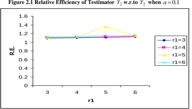
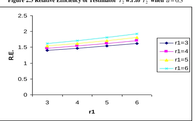
Table 2.1 to 2.4, represents the relative efficiency of the estimator Y₂' with respect to Y₂ for a = .1(.1).4,



1

r

3,4,5,6,

r

₂



3, 4, 5, 6.The figure 2.1 to 2.4 shows that for small values of a and for smaller values of

r

₁,

2

REFERENCES

[1] Bancroft, T.A. (1944) “On biases in estimation due to the use of preliminary test of significance.Ann.Math.Stat.15, 190-204.

[2] Bhattacharya, S.K and Srivastava, V.K. (1974) “A preliminary test procedure in life testing”. Jour.Amer.Stat.Assoc. 69,726-729.

[3] Cohen A. (1965) “Estimates of linear combination of the parameters in the mean vector of a multivariate distribution.”Ann.Meth.stat.36, 78-87.

[4] Epstein, B and Sobel, M (1953) “Life Testing.”Jour. Amer.Stat. Assoc. 48,486-507.

[5] Han, C.P., Rao.C.V. and Ravichandran, J.(1988) “ Inference based on conditional specification.” A second bibliography. Comm. Stat. Theo.Meth.A176, 1-21.

[6] Hirano, K. (1973) “Biased efficient estimator utilizing some apriori information,” Jour.Japan Stat.Soc 4, 11-13.

[7] Hogg, R.V. (1974) “Adaptive robust procedures: A partial review and some suggestions for future applications and theory.” Jour.Amer.Stat.Assoc.69, 909-923.

[8] Katti, S.K. (1962) “Use of some apriori knowledge in the estimation of mean from double samples.”Biomatrics 18,139-147.

[9] Pandey, B.N. (1977) “Testimator of the scale parameter of the exponential distribution using Linex loss function.” Comm.Sta.Theo.Meth.26, 2191-2200.

[10] Pandey, B.N.and Malik, H.J. (1994) “Some improved estimators for common variance of two populations.” Comm.Stat.Theo.Meth, 23(10), 3019-3035.

[11] Pandey, B.N.and Singh, J. (1977a) “Estimation of variance of normal population using apriori information.”Jour.Ind.Sta.Assoc.15, 141-150.

[12] Pandey, B.N.and Singh, J. (1977b) “A note on the estimation of variance in exponential density.” Sankhya 39,294-298.

[13] Sinha, S.K. (1986) “Reliability and life testing.” Wiley Eastern Ltd., New York.

[14] Sinha, S.K.and Kale, B.K. (1980) “Life testing and Reliability estimation.” Wiley Eastern Ltd., New York.

[15] Srivastava, S.R. (1976) “A preliminary test estimator for the variance of a normal distribution.” Jour.Ind.Sta.Assoc.19, 107-111.

[16] Varian, H.R. (1975) “A Bayesian approach to real estate assessment.” In studies in Bayesian econometrics and statistics in honor of L.J.Savage, Eds S.E.Feinberge and A, Zellner, Amsterdem North Holland, 195-208.

APPENDICES

Figure 2.1 Relative Efficiency of Testimator Y₂'w.r.to Y₂ when a0.1

0 0.2 0.4 0.6 0.8 1 1.2 1.4 1.6

3 4 5 6

r1

R

.E

.

Figure 2.2 Relative Efficiency of Testimator Y₂'w.r.to Y₂ when a0.2

1.1 1.15 1.2 1.25 1.3 1.35 1.4 1.45

3 4 5 6

r1

R

.E

.

r1=3

r1=4

r1=5

r1=6

Figure 2.3 Relative Efficiency of Testimator Y₂'w.r.to Y₂ when a0.3

0 0.5 1 1.5 2 2.5

3 4 5 6

r1

R

.E

.

r1=3

r1=4

r1=5

r1=6

Figure 2.4 Relative Efficiency of Testimator Y2'w.r.to Y2 when a0.4

0 0.5 1 1.5 2 2.5 3 3.5 4

3 4 5 6

r1

R

.E

.

r1=3

r1=4 r1=5