A Modified Particle Swarm Optimization Algorithm

(1)

A Modified Particle Swarm Optimization

Algorithm

Jinrong Zhu

School of Business Administration, North China Electric Power University, Beijing 102206,China Email: [email protected]

Abstract—A modified particle swarm optimization

algorithm is proposed in this paper. In the presented algorithm, every particle chooses its inertial factor according to the approaching degree between the fitness of itself and the optimal particle. Simultaneously, a random number is introduced into the algorithm in order to jump out from local optimum and a minimum factor is used to avoid premature convergence. Five well-known functions are chosen to test the performance of the suggested algorithm and the influence of the parameter on performance. Simulation results show that the modified algorithm has advantage of global convergence property and can effectively alleviate the problem of premature convergence. At the same time, the experimental results also show that the suggested algorithm is greatly superior to PSO and APSO in terms of robustness.

Index Terms—particle swarm optimization, modified

particle swarm optimization, function optimizing

I. INTRODUCTION

Particle swarm optimization (PSO) algorithm [1], which is proposed by James Kennedy and Russell Eberhart in 1995, comes from the research on the predatory behaviour of birds and is a branch of swarm intelligence. PSO is a kind of algorithm whose optimal solutions are searched by collaborating between every individual and has been applied in many fields [2], such as function optimizing and ANN training, because of its simple concept and high efficiency.

As the other global algorithms, PSO takes the risk of including premature convergence and vibration in the late iteration. To promote the performance of the PSO algorithm, some improved PSO algorithms are proposed [3-6]. Shi Y and Eberhart R C suggested controlling the influence of the former velocity on current velocity by using inertial factor [3] . First of all, a bigger inertial factor is used to confirm the approximate position of the optimal solution rapidly. Then, a smaller inertial factor is used to perform refined local search. Because of the shortcoming of the modified algorithm in the search in complicated problems, Shi Y and Eberhart R C suggested changing dynamically the inertial factor by Fuzzy Controller [4]. But the fuzzy adaptive particle swarm optimization is difficult to implement because of some

requirements of the pre-know about some characteristics of the problem. A new adaptive particle swarm optimization algorithm is developed in our study [7]. In the algorithm, every particle chooses its inertial factor according to the fitness of itself and the optimal particle.

In this paper, along with the idea that a particle chooses its inertial factor according to the approaching degree between the fitness of itself and the optimal particle, a modified particle swarm optimization algorithm is suggested. In the proposed algorithm, a random number is introduced into the algorithm in order to jump out from local optimum and a minimum factor is used to avoid premature convergence. Lots of experiments show that the proposed algorithm is more effective than PSO and APSO.

The rest of the paper is organized as follows. Section 2 introduces the general description of PSO algorithm. Section 3 presents the modified PSO algorithm. Section 4 discusses the experimental results. And section 5 concludes.

II.PARTICLE SWARM OPTIMIZATION (PSO)ALGORITHM

In the particle swarm optimization (PSO) algorithm, every solution of the optimization problem is regarded as a bird in the search space, which is called particle. Every particle has a velocity by which the direction and distance of the flying of the particle are determined, and a fitness that is decided by the optimized function. The particles search in the solution space by pursuing the optimal particle currently.

In the process of PSO optimization, a group of random particles (random solutions)are given by initializing, and then the optimal solution is obtained by iterative process. In each iteration, a particle updates itself by tracking two extreme values, which are personal best solution (p) and global best solution (g). The personal best solution (p) is the optimal solution that was found by the particle itself, and the global best solution (g) is the optimal solution that was found by the population. After the two extreme values are discovered, every particle updates its velocity and position based on

) ( )

( ₂ ₂

1 1

1 k k k k k

k wv cr p x c r g x

v ₊ = + − + − (1)

1

1 +

+ = k + k k x v

x (2) where vk and xk are velocity vector and position of the particle currently, pk and gk denote the position of the optimal solutions that was found by a particle itself and the whole particle swarm, w is a nonnegative inertial Manuscript received March 20, 2009; revised May 15, 2009;

accepted June 15, 2009.

(2)

factor, c1 and c2 are learning parameters, r1 and r2 are random number from 0 to 1. The velocity of the particle is often limited on each dimension generally. When the updated velocity exceeds the max value vmax that is pre-set, it should be changed to vmax.

III.A MODIFIEDPARTICLE SWARM OPTIMIZATION

ALGORITHM

A. The adjustment of the inertial factor

In this paper, a modified approach to adjusting the inertial factor adaptively is proposed based on lots of experiments.

First, every particle chooses its inertial factor according to the approaching degree between the fitness of itself and the optimal particle. A particle with better fitness chooses a smaller inertial factor and a particle with worse fitness chooses a bigger inertial factor. Taking the strategy, the proposed algorithm will search in large range in the early iterations so that the approximate location of the optimal solution is confirmed rapidly and search in small range in the late iterations in order that the exact solution is found.

Secondly, a random number is introduced into the algorithm in order to jump out from local optimum.

Finally, a minimum factor is used to avoid premature convergence.

Facing on a minimization problem, the inertial factors of the particles are updated according to Eq.(3) and Eq.(4). min min f f f k

w_p=ε − (3)

⎩ ⎨ ⎧ > = other if 0 0 w w w w

w p p (4)

where f is the fitness of the current particle, fmin is the fitness of the optimal particle currently; k is a parameter by which the average inertial factor of all particles is controlled. ε is a random number from 0 to 1. wp is the minimum of the factors that is pre-set so that the risk of the premature convergence is reduced.

B. The procedures of the modified algorithm

The optimization procedures of the modified PSO (MPSO) are given as follows.

(1) Generate randomly the initial position and velocity of the particles.

(2) Calculate the fitness of each particle.

(3) Calculate personal best solution (p) and global best solution (g), then search a better position by iteration based on formulas Eq.(1) and Eq. (2), where the w will be gained based on Eq. (3) and Eq.(4).

(4) Repeat from (2) to (3) until the halt criteria are met. The pseudocode for MPSO algorithm is as follows.

begin

initialize the population

while (termination condition = false) do

for ( i = 1 to number of particles)

evaluate the fitness : = f(x) update p and g

increase i

for ( i = 1 to number of particles) calculate the new inertial factor : = wp if wp>w0

w = wp else

w = w0 end if

calculate vk+1 and xk+1 increase i

end do end

IV.SIMULATIONSTUDY

A. Benchmarks

Five well-known benchmarks were used to evaluate the performance, which were commonly used in evolutionary optimization methods and widely used in evaluating performance of PSO methods. All benchmarks used are listed as follows.

f1: Sphere function

∑

= = n i i x x f 1 2

1( ) (5)

f2: Rosenbrock function

∑

= + − + − = n i i i

i x x

x x f 1 2 2 2 1

2( ) 100( ) ( 1) (6)

f3: Rastrigin function

∑

= + − = n i i i x x x f 1 2

3( ) ( 10cos(2π ) 10) (7)

f4: Griewank function

1 ) cos( 4000 1 ) ( 1 1 2

4 =

∑

−

∏

+

= = n i n i i i i x x x

f (8)

f5: Schaffer's f6 function

[

₂

]

2

2 2 1 2 2 2 1 2 5 1 ) ( * 001 . 0 5 . 0 sin 5 . 0 ) ( + + + + − = x x x x x

f (9)

Simulations were carried out to find the global minimum of the every function. The performance of the MPSO method is compared with the standard PSO method and adaptive particle swarm optimization (APSO).

B. Performance criteria

The optimization performance is evaluated using following statistics, namely, Average best fitness (ABF), Standard deviation (SD), Mean Iteration (MI), Min Iteration (MINI), Fail Number (FN). All statistics are calculated according to Eq.(10) ~ Eq.(14).

(3)

∑

=

= n

i i

I n MI

1 1

(12)

) min(Ii

MINI= (13)

∑

=

= n

i i

F n FN

1 1

(14)

Where n is the number of the trials, fi is the best fitness of the ith trial, Ii is the iteration that the algorithm meets the convergence criteria that are pre-set. Fi = 0 or 1. If an algorithm cannot meet the pre-set convergence criteria after the maximum iteration, we think that the algorithm is fail and Fi is set to 1 and Ii is set to 1.2 times of the max iteration, else Fi is set to 0.

ABF and MI are the measure of the mean performance, and SD and FN are the indexes that measure the robustness. The smaller ABF and MI mean an algorithm is more effective. The smaller SD and FN denote that an algorithm is more robust. MINI is a reference value who expresses the minimal iteration when a trial converges more rapidly than all other trials.

C. Parameters selection

Table I shows the parameters of the test functions including the range of the search and the maximum velocity.

TABLE I. PARAMETERSFORTESTFUNCTIONS

Function Search Range Vmax

Sphere function (f1) (-100,100)n 20

Rosenbrock function (f2) (-100,100)n 20

Rastrigin function (f3) (-10,10)n 2

Griewank function (f4) (-600,600)n 120

Schaffer's f6 function (f5) (-100,100)n 20

The five benchmarks were tested with the dimensions 2, 4 and 6 (only 2-dimension is tested for f5). In this paper, the population size is set to 30, and the parameters c1, c2 are set to c1=c2=1.

In the standard PSO, the inertia weight is set to 0.9. In the APSO, the inertia weight is scaled linearly from 0.9 to 0.4.

D. Performance analysis

In the study, the optimum solutions after a predefined number of iterations are investigated. For each function, 20 trials were carried out and the average best fitness and the standard deviation are calculated.

In the MPSO, the parameter k is set to 1.

Given dimension (D.) and maximum generation (Gen.), the average best fitness and standard deviations are summarized in Table II.

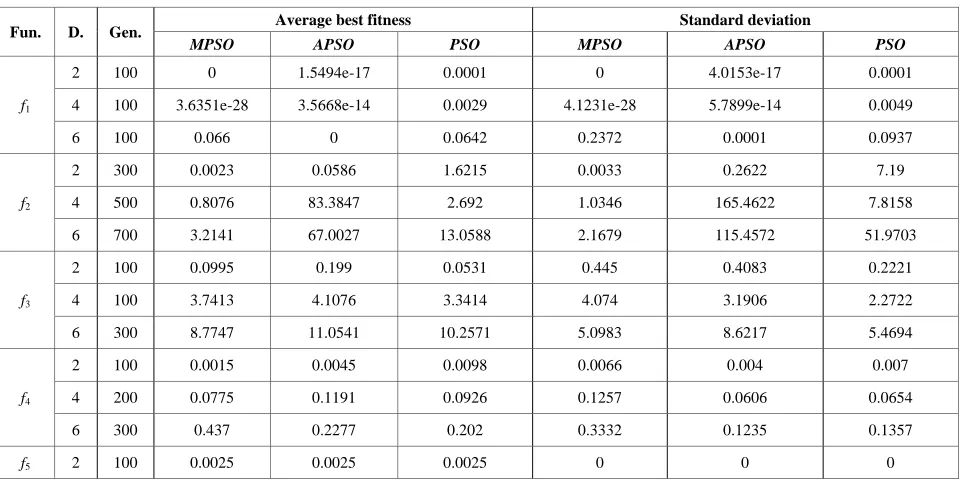
In the Table II, we can find that

1) In all 13 cases, there are 10 times that MPSO has gained smaller ABF than APSO and 8 times that MPSO has smaller ABF than PSO. A smaller ABF indicates that the algorithm is more effective, so we can conclude that the MPSO is superior to APSO and PSO.

2) For all cases, there are 6 times that MPSO has got smaller SD than APSO and 7 times that MPSO has obtained smaller SD than PSO. At the same time, MPSO performs as well as APSO and PSO for function f5 if the SD is considered as measurement. A smaller SD means an algorithm is more robust. So we can conclude that MPSO is slightly robust than PSO and as robust as APSO. Fig.1~Fig.5 show the average fitness value (AFV) through 20 times experiments for all functions with 2 dimensions.

In the Fig.1, Fig.2, Fig.4 and Fig.5, the MPSO converges more rapidly than the standard PSO and APSO. Only in the Fig.3, MPSO converges slower than PSO and more rapid than APSO. They denote that MPSO can converge faster than PSO and APSO in summary.

TABLE II. COMPARISONSOFTHEPERFORMANCES

Fun. D. Gen. Average best fitness Standard deviation

MPSO APSO PSO MPSO APSO PSO

f1

2 100 0 1.5494e-17 0.0001 0 4.0153e-17 0.0001

4 100 3.6351e-28 3.5668e-14 0.0029 4.1231e-28 5.7899e-14 0.0049

6 100 0.066 0 0.0642 0.2372 0.0001 0.0937

f2

2 300 0.0023 0.0586 1.6215 0.0033 0.2622 7.19

4 500 0.8076 83.3847 2.692 1.0346 165.4622 7.8158

6 700 3.2141 67.0027 13.0588 2.1679 115.4572 51.9703

f3

2 100 0.0995 0.199 0.0531 0.445 0.4083 0.2221

4 100 3.7413 4.1076 3.3414 4.074 3.1906 2.2722

6 300 8.7747 11.0541 10.2571 5.0983 8.6217 5.4694

f4

2 100 0.0015 0.0045 0.0098 0.0066 0.004 0.007

4 200 0.0775 0.1191 0.0926 0.1257 0.0606 0.0654

6 300 0.437 0.2277 0.202 0.3332 0.1235 0.1357

(4)

0 10 20 30 40 50 60 70 80 90 100 -70

-60 -50 -40 -30 -20 -10 0 10

Number of Iterations

A

v

er

age F

it

nes

s

V

al

ues

(l

og)

PSO APSO MPSO

Figure 1. Average fitness values for f1 (n=2).

Figure 2. Average fitness values for f2 (n=2)

Given dimension (D.), maximum generation (Gen.) and error criteria (Err.), The MI, MINI and FN of 20 trials are calculated out. When setting error criteria, a more complex function will have bigger error value.

The MI, MINI and FN are listed in Table III. In the Table III, we can find that

1) In all 13 cases, there are 12 times that MPSO has gained smaller MI than APSO and 13 times that MPSO has smaller MI than PSO. A smaller MI indicates that the algorithm can converge more rapidly, so we can conclude that the MPSO is superior to APSO and PSO.

2) For all cases, there are 11 times that MPSO has not got bigger FN than APSO and 12 times that MPSO has not expressed worse than PSO when the FN is considered as measurement. A smaller FN means an algorithm is more robust. So we can conclude that MPSO is more robust than PSO and APSO.

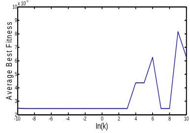
E. The influence of the parameter k on performance In the proposed algorithm, parameter k could have some influence on performance. In this paper, the performance of the suggested method is checked with different k. For all test functions, the changes of the average best fitness are illustrated in Fig.6~Fig.10 (only 2-dimension functions are illustrated).

As shown in the Fig.6~Fig.10, the algorithm performance is rather stable when the parameter k is not bigger than 1 (i.e. e0). We can also find that the performance is often different when the k is bigger than e2. It means that the proposed algorithm is rather robust when the parameter k is controlled to not bigger than 1.

Figure 6. The influence of the parameter k on performance for f1 (n=2)

0 10 20 30 40 50 60 70 80 90 100

-3 -2 -1 0 1 2 3

A

v

e

rage Fi

tnes

s

V

a

lues

(l

og)

PSO APSO MPSO

0 10 20 30 40 50 60 70 80 90 100

-7 -6 -5 -4 -3 -2 -1 0 1 2

A

v

e

rage F

it

nes

s

V

a

lues

(l

og)

PSO APSO MPSO

0 10 20 30 40 50 60 70 80 90 100

-7 -6 -5 -4 -3 -2 -1

A

v

er

ag

e F

it

ne

s

V

al

u

es

(l

og

)

PSO APSO MPSO

-10 -8 -6 -4 -2 0 2 4 6 8 10

-1 -0.5 0 0.5 1

In(k)

A

v

er

age B

es

t

F

it

ne

s

0 50 100 150 200 250 300

-10 -5 0 5 10 15

A

v

er

ag

e F

it

ne

s

V

al

ues

(l

og)

(5)

TABLE III. COMPARISONSOFTHEPERFORMANCES

Fun. D. Gen. Err. Mean Iteration Min Iteration Fail Number

MPSO APSO PSO MPSO APSO PSO MPSO APSO PSO

f1

2 100 0.0001 19.1 40.05 74.1 8 7 7 0 0 4

4 100 0.0001 29.95 55.05 108.95 16 49 89 0 0 19

6 100 0.0001 41.8 70.65 110 18 59 110 2 1 20

f2

2 300 0.01 116.8 99.05 163.35 32 42 40 0 1 4

4 500 5 34.5 283.9 187.6 12 23 32 0 8 3

6 700 10 33.45 357.95 256.85 18 41 65 0 8 1

f3

2 100 0.01 31.35 49.4 52.7 9 19 8 1 4 2

4 100 10 17.25 18.95 22.35 5 8 7 1 1 0

6 100 20 11.2 29.25 34.2 8 11 7 0 2 2

f4

2 100 0.01 38.6 55.6 84.45 9 8 25 1 0 10

4 200 0.5 14.75 24 28.4 9 10 6 0 0 0

6 300 2 9.25 10.3 10 5 8 7 0 0 0

f5 2 100 0.005 13.85 17.1 17.95 5 5 5 0 0 0

-100 -8 -6 -4 -2 0 2 4 6 8 10

2 4 6 8 10 12

In(k)

A

v

er

ag

e B

es

t F

it

nes

s

-100 -8 -6 -4 -2 0 2 4 6 8 10

0.005 0.01 0.015 0.02 0.025 0.03

In(k)

A

v

er

ag

e B

es

t F

it

nes

s

-100 -8 -6 -4 -2 0 2 4 6 8 10

0.2 0.4 0.6 0.8 1

In(k)

A

v

er

age B

es

t

F

it

ne

s

-102 -8 -6 -4 -2 0 2 4 6 8 10

3 4 5 6 7 8 9 10x 10

-3

In(k)

A

v

er

ag

e B

es

t F

it

nes

(6)

V.CONCLUSION

In this paper, a modified particle swarm optimization algorithm is proposed. In the presented algorithm, every particle chooses its inertial factor according to the approaching degree between the fitness of itself and the optimal particle. Simultaneously, a random number is introduced into the algorithm in order to jump out from local optimum and a minimum factor is used to avoid premature convergence. Five well-known functions are chosen to test the performance of the suggested algorithm and the influence of the parameter on performance. The simulation results show that the MPSO algorithm is superior to the standard PSO and APSO.

ACKNOWLEDGMENT

This work was supported in part by a grant from North China Electric Power University (No.200822047).

REFERENCES

[1] KENNEDY J, EBERHART R C. “Particle swarm

optimization”. Proc of IEEE Int Conf on Neural Networks. Piscataway, NJ: IEEE Press, 1995, pp.1942-1948.

[2] Eberhart R C, Shi Y H. “Particle swarm optimization: developments , applications and resources”. Proceedings of the IEEE Congress on Evolutionary Computation. Piscataway, USA: IEEE Service Center , 2001,pp. 81-86. [3] Shi Y, Eberhart R C. “A modified particle swarm

optimizer”. IEEE International Conference of Evolutionary Computation, Anchorage, Alaska, May 1998,pp.69-73

[4] Shi Y, Eberhart R C. “Fuzzy adaptive particle swarm optimization”. Proceedings of the Congress on Evolutionary Computation. Seoul, Korea, 2001,pp.101-106 [5] LI Yonggang, GUI Weihua, YANG Chunhua, CHEN

Zhishen, “A resilient particle swarm optimization algorithm”, Control and Decision, 23,2008(1),pp. 95-98 (in Chinese)

[6] Lu Zhensu, Hou Zhirong, “Particle swarm optimization with adaptive mutation”, ACTA electronica sinica. 32,2004(3),pp.416-420 (in Chinese)

[7] Zhu Jinrong, Zhao Jianbao, Li Xiaoning. A New Adaptive Particle Swarm Optimization Algorithm, 2008 International Workshop on Modelling, Simulation and Optimization, pp.456-458