Initialization of Weights in Deep Belief Neural Network Based on Standard Deviation of Feature Values in Training Data Vectors

(1)

Initialization of Weights in Deep Belief Neural

Network Based on Standard Deviation of Feature

Values in Training Data Vectors

Nader Rezazadeh

Department of Computer / Science and Research Branch of, Islamic Azad University, Tehran, Iran

Abstract - Nowadays, the feature engineering approach has become very popular in deep neural networks. The purpose of this approach is to extract higher-level and more efficient features compared to those of learning data and to improve the learning of machines. One of the common ways in feature engineering is the use of deep belief networks. In addition, one of the problems in deep neural networks' training is the training process. The problems of the training process will be further enhanced in the event of an increase in the dimensions of the features and the complexity of the relationship between the initial features and the higher-level features. In the present paper, we attempt to set the initial weights based on the standard deviation of the feature vector values. Hence, a part of the training process is initially conducted and a better starting point can be provided for the weight training process. However, the impact of this method, to a large extent, depends on the relationship between the training data itself and the degree of independence of the training data's feature values. Experiments conducted in this field have achieved acceptable results.

Keywords - Neural Network; Restricted Boltzman Machine; Deep Belief Network

1. Introduction

eural network is one of the most important tools in the process of classification and data regression [1]. Nowadays, neural networks are used in areas such as audio processing, video imaging, and texts. The increase in the complexity of classifications requires an increase in the order of the neural network relationship through increasing the number of layers of a network which, in turn, has a complicated computational increase [1]. This computational complexity and the large space of parameters have led the commonly used methods in neural networks to use less large numbers of layers [2]. In addition to the low speed of training, the problem of the large number of layers in these types of networks, is the presence of local minima, which in most cases does not lead us to a desirable outcome. One of the solutions to this problem is to use the deep belief networks [3], DBN, which allow for the creation of networks with a large number of layers [3].

deep belief networks' layers are constructed from limited Boltzmann machine [3] or 2RBM/ Every limited Boltzmann machine is a generative and non-directional probability model [4] that uses a hidden layer to model a distribution on its visible variables. In fact, by placing limited Boltzmann machines on one another, we can create deep neural networks for hierarchical processes. Therefore, most of the changes and enhancements lead to the improvement of these networks and in effect to the correction of limited Boltzmann machines. The use of deep

belief networks is not only applicable to categorization tasks, but also, it can be used as a feature extraction method. For this reason, many of the work done in developing machine learning algorithms tend to preprocessing, feature extracting, and feature learning. Feature learning attempts to use the input data to create a system for extracting the feature, so that its output is used for classification and other applications. The benefits of deep belief networks in feature learning is that, with the help of unsupported data, the networks can extract high-level features of educational data [5] and increase the power of differentiation between different classes of data [6]. But the use of the deep belief networks involves some problems as well. The most important problem is the training of weights and the extraction of high-level features in each layer of the deep belief network. Nowadays, sampling method of Gibbs [7] and contrastive divergence [8] are proposed to serve the purpose. The long training process in Gibbs sampling method and the inadequate accuracy of the contrastive divergence training process have proved the need to improve the training process. An important step in improving the training process is to select the appropriate initial values. The initial values of weights are typically randomly selected [9]. Hence, a new approach is considered in this paper for the initial selection of weights. Rest of the paper is organized as follows, Section II contain the Literature Review of DBN, Section III contain the Suggested Method, Section IV contain the experimental results and finally, section V concludes

research work.

(2)

2. Literature Review

Today, unsupervised statistical models are considered as an appropriate tool for extraction of the features and classification of audio, imaging, and statistical data [8]. Here the bracket represents the calculation of expected value on the multiplication of the hidden and visible unit values. Thus, with this derivative, we can easily obtain the law of weight modification of in the probability log for the training data as follows [10]. Where is the learning rate. Similarly, we can write the weight modification law in the bias parameters [10].

Restricted Boltzmann machines (RBMs) have been used as generative models of many different types of data[8]. Restricted Boltzmann machines were developed using binary stochastic hidden units. A Restricted Boltzmann Machine (RBM ) [10] is a network of symmetrically coupled stochastic binary units. It contains a set of visible units ∈{0,1} and a set of hidden units ℎ∈{0,1}𝑃. a RBM is an Markov Random Field associated with a bipartite undirected graph. It consists of visible units

=( 1,…, ) representing the observable data, and hidden units 𝐻=(𝐻1,…,𝐻 for computing the dependencies between the observed variables. the random variables ( ,𝐻) take the values ( ,ℎ)∈{0,1} + . a RBM model shown in Figure 1[10].

Figure 1. The undirected graph of an RBM with n hidden and m visible variables[9]

Where , ℎ are the binary states of visible unit and hidden unit , and , are their biases. is the weight between them. Deep Belief Net(DBN)[11] , is a hybrid generative model .at DBN, multiple layers are learned as layer-by-layer way, the resulting composite model is a multilayer Boltzmann machine. deep belief net has undirected connections between its top two layers and downward directed connections between all its lower layers. In a restricted Boltzmann machine, state power {v, h} is defined in exchange for the restricted Boltzmann

machine with the distribution of θ as follows [12].

, ℎ; 𝜃 = (1 − ∑

∈

− ∑ ℎ −

∈ℎ

∑ ℎ ,

The value of joint probability model for the event of paired vector , ℎ being based on the energy function is described in the following [12].

𝑃 , ℎ = −𝐸 ,ℎ In the above equation, Z is given by summing over all possible pairs of visible and hidden vectors [12].

= ∑ −𝐸 ,ℎ ,ℎ

Z Also Called "partition function". The probability that the network assigns to a visible vector, v, is given by summing over all possible hidden vectors [12].

𝑃 = ∑ −𝐸 ,ℎ ℎ

A. RBM Training

In a restricted Boltzmann machine θ, the amount of log likelihood for a single training vector v is defined as equation (5) [12].

ℒ

𝜃| = 𝑃 |𝜃

= ln ∑ −𝐸 ,ℎ ℎ

− ∑ −𝐸 ,ℎ

,ℎ

To adjust the weights of , , , for a vector v, through the gradient descent method, derived Log-Likelihood is calculated in proportion to [12].

ℒ 𝜃|

=

− ∑ 𝑃 ℎ| , ℎ

ℎ

+ ∑ 𝑃 , ℎ , ℎ ,ℎ

= ∑ 𝑃 ℎ| ℎ − ∑ 𝑃 ∑ 𝑃 ℎ| ℎ ℎ

ℎ

= 𝑃 𝐻 = | − ∑ 𝑃 𝑃 𝐻 = |

Probability of the ith hidden node to equal one in the

graphic restricted Boltzmann machine model being based on observable vector v is called 𝑃(𝐻=1| ). The value of P 𝑃(𝐻=1| )Is calculated based on the values of ith feature

(3)

∑ ∊ 𝜕 ℒ 𝜃|_𝜕 =

7

𝐿 ∑[− 𝑃 ℎ| [ , ℎ ] + 𝑃 ℎ, [ , ℎ ]] ∊

𝐿∑ [−∊ 𝑃 ℎ| [ ℎ ] + 𝑃 ℎ, [ ℎ ]] =< ℎ >𝑃 ℎ| −< ℎ >𝑃 ℎ,

Parameter L is the number of training vectors ∈ . In equation (7), the normalized constant Z is common in probability values of P ℎ| ) and P ℎ,v . With q denoting the empirical distribution, equation (8), Gives us often stated below equation (8) [13].

∑ ℒ 𝜃| ∊

∝ < ℎ > − < ℎ >

Since there are no direct connections between the hidden units, these units are separated observing the visible units' condition. Thus, having the values of visible units , the binary state of ℎ for each hidden unit –j- takes the value of 1 with the probability below [14].

∆w =∈ (< ℎ > −< ℎ > )

Thus, < ℎ > is easily calculated by obtaining the values of ℎ .

∆a =∈ < > −< > ∆b =∈ < ℎ > −< ℎ >

Also, since there are no direct connections between visible units, one can calculate the visible unit i of mode

as follows- provided that the mode vector of the hidden units of the model ℎ atais obtained [14].

𝑃(ℎ = | ) =

+ exp −( + ∑ )

,

the binary state of for each visible unit –i- takes the value of 1 with the probability below [14].

𝑃( = |ℎ ) =

+ exp −( + ∑ ℎ ) ,

the binary state of ℎ for each hidden unit –j- takes the value of 1 with the probability below [14].

𝑃(ℎ = | ) =

+ exp −( + ∑ )

,

Obtaining the value of < ℎ> is a little more complicated. To calculate this value, we must start a random value in visible units and implement the Gibbs sampling for a long time. However, due to the impossibility of this method and its long execution time, another method is used called contrastive divergence [15].

3. Methodology

In the suggested method, we try to determine the initial values of weights based on the behavior of the features of the nodes. In this method, it is attempted to determine the initial values of the connected edges of the hidden layer to a feature based on the average change in the values of a feature versus the mean of the feature or standard deviation. To illustrate this relationship, we first want to

examine the relative role of the changes in the value of the features in the weight training process. To achieve this objective, all probability functions are written in terms of

ata_{to examine the effect of changes in the values of the} features of the training data vectors on the weight changes. The value of 𝑃( = |ℎ ) is easily calculated based on ata. It suffice to put equation (11) in equation (12). As a result, the equation (14) is obtained

(4)

𝑃( = |ℎ ) =

+EXP − + ∑

+EXP(− + ∑ )

,

By putting the above equation in the equation (13), the expression of 𝑃(ℎ = | ) will be equal to equation (15).

𝑃(ℎ = | ) =

+ exp − + ∑

( + exp − + ∑ + exp(− + ∑ ) )

In this part, we will consider the weight changes in terms of ∆ = [ ℎ ] − [ ℎ ]. Suppose the

` feature of the input data vector being ,

expression 𝑃(ℎ = | ) can be rewritten as equation (16).

𝑃(ℎ = | ) =

+ −( + +∑`= , `≠ ` ` )

ℎ ` , , ` ≠i

If _`= , equation (16) can be written as equation (17).

𝑃(ℎ = | ) =

+ (− + +∑`= , `≠ ` ` )

Accordingly, the value of [ _`ataℎ ] will be equal to equation (18).

[ `ataℎ ] = × ₊ ₍₋ ₊

+∑`= , `≠ ` ` )

By placing equation (18) in (14) and (15), the value of [ ` ℎ ] will equal to equation (19).

[ ` ℎ ] =

( + exp − + ∑ + exp − + +∑`= , `≠ ` ` ₎

×

+ exp − + ∑

( + exp − + ∑ + exp − + +∑`= , `≠ ` ` ₎

(5)

Given that the following inequality is established in a logic sigmoid function [16].

∀ , →

+ exp( )

And regarding that ∀x,

+ x < , equation (21) can be deduced.

( + exp − + ∑ + exp(− + ∑ ) )

+ exp −( + ∑ )

And in a similar way the equation below can be deduced.

+ exp

( − + ∑

( + exp − + ∑ + exp(− + ∑ ) ) )

+ exp − + ∑ _{+ exp(−} _{+ ∑} ₎

Given the above equations of (20) and (21), it can be concluded that if _`ata= , then the relationship

[ àtaℎ ] [ ` ℎ ] is correct. Therefore, if àta= , then the equation (22) is established. ∆W` = [ àtaℎ ] − [ ` ℎ ]

When considering this issue, one might say that if i feature is equal to 1, then ∆W value moves toward the increasing of the weight of wij. This is to increase the relationship

between the feature _` and the hidden layer. By doing this, the energy level of the hidden layer is decreased in comparison to the training vector in proportion of the total energy, and conversely, the probability of generating training data is increased through the model. If we consider

this relationship _`ata= , equation (23) can be concluded.

∆W` = [ × ℎ ] − [ ` ℎ ] ∆W` = −[ ` ℎ ]

Given the equations (20) and (21) and (22), the value of ∆W_` will be equal to equation (24).

∆W` = − × [ ` ℎ ] =

+ exp − + ∑ _{+ exp −} ₊

+∑`= , `≠ ` `

×

+ exp − + ∑

( + exp − + ∑ + exp − + +∑`= , `≠ ` ` ₎

Given that ∀ , / + exp , this relation ∆W` < will definitely be established. As an

(6)

direction of weight of _` on the edge. This is to increase the weights between the node of i` in the visible layer and the hidden layer. Hence, when the value of i` feature in the training data vectors becomes 0 or 1, the gradient function will have 2 different approaches in the adjustment of weights. The gradient function moves in one direction to gain weight on the node of i` and the hidden layer, and the other one moves to lose weight.

The more the other values of feature vectors be closer to each other, the sum of the decreases and the increases inclines more to zero. Because the sum of the decreasing values and the sum of the increasing values equal to zero. Regarding the above issues, the initial values of the edges of the hidden layer connected to a feature can be determined based on the average change of the values of feature relative to the mean of feature values or standard deviations. The purpose of this initialization is to determine the best starting point for weight training. The high standard deviation of a values feature refers to a great change in the values of that feature. This reduces the gradient and, consequently, reduces the value of ∆ _` . Initially, the standard deviation of the feature values of the ith node is defined as follows.

𝜎vi`= √∑ (

∑L_l= v_i`l

L ) − (v`) L

= 5

ℎ 𝐿 , ′

The L parameter represents the number of training data, and n indicates the number of features. The standard deviation values need to be normalized in order to determine the values of weights between zero and one. Thus, we have to use equation (26) [17].

𝜎v𝑁i` 𝑧 =

𝜎vi`

vi`

ℎ vi`=

∑ vL= `

L , 𝐿 , ′

vi` in equation (26), is equal to the mean value of the

feature i`. As already mentioned, in the suggested method, the initial values of weights are inversely related to the standard deviation of values. Therefore, − d̅̅̅̅_v_i is used to determine the initial values of weight.

= |∑L=_{L | ×}v` − (𝜎v𝑁i` 𝑧 )

If the mean value of i` is low, the correlation with the hidden layer will not be meaningful - even with a low standard deviation. Because the received values by the corresponding feature will be considered as negligible by the hidden layer. Therefore, the standard deviation of

values alone cannot be regarded as a criterion. In the following, it is necessary to multiply the mean value of the feature i` by the standard deviation of the values of the i` feature. In this method, the relationship between the values of the features is not considered in the determination of the initial weights. In the process of training, if there is a relative correlation between the values of the features, the weight values are corrected. In many cases, the values of all the features are not completely related; thus, the weight values cannot be changed significantly.This means that we are a part of the training process at the same initialization stage. But when the relationship between the values of a property and other features is established, the initial weights determined by this method will definitely change. The amount of these changes depends on the relationship between the values of the feature.

4. Results and Discussion

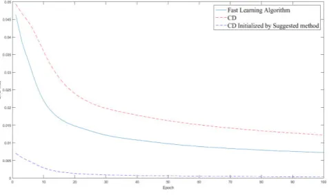
In this section, two different data sets are selected to examine the success rate of the proposed method. Since this method is based on the standard deviation of the features, two sets of data have been selected having a significant difference in the standard deviation of their features. One of the selected datasets, is the dataset of car pricing [18]. The other dataset used in the research is the Heart Disease data set [19]. The amount of standard deviation of the features in the heart disease dataset is 0.081, while this value is 0.23 in the car pricing dataset. The average standard deviation of the features in the car pricing dataset is so much higher than that of the heart disease dataset. 75% of the data was used for training and 25% of the data was used for testing in the experiments. In addition, the Fast Learning Algorithm [20] method was used along with the CD method and the initialization-based CD method as the proposed method. In Figure 2, the mean square of the deep neural network's training error is given for the mentioned training algorithms. The implementation of these algorithms is based on car pricing data.

Figure 2. MSE Error of Contrastive Divergence, Contrastive Divergence Initialized by Suggested method And fast training Algorithm

for car Data set

(7)

performance. The proposed method has lower mean square of training data error, especially in the initial education courses. The existence of a low standard deviation in the values of each feature has led to the superiority of the proposed training algorithm. The heart disease dataset is used in the next experiment, to test the proposed algorithm according to the new data with different statistical characteristics. In Figure 3, the mean square of the deep belief network's training error is presented for the CD training algorithms, the CD initialized by the proposed method and the fast learning algorithm [20].

Figure 3. MSE Error of Contrastive Divergence, Contrastive Divergence Initialized by Suggested method And fast training Algorithm

for Heart Disease Data set

Unlike the previous experiments, in the current experiment, the mean square of the training error of the initialization -based CD algorithm – the proposed method was better than the fast learning algorithm. The superiority of the fast learning algorithm is evident in all courses. The reason is the high mean standard deviation of the values of each feature in the heart disease dataset. This issue has caused the inability of the CD training algorithm in using the proposed method's capability in the determination of the initial values of weights. In the following, the chart of percentage accuracy of the deep belief network being based on the training algorithms is presented in Figure 4, based on the car pricing data set.

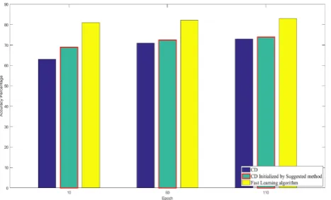
Figure 4. Accuracy Percentage of Contrastive Divergence, Contrastive Divergence Initialized by Suggested method and fast training Algorithm

In this experiment, the validity of the proposed training algorithms was evaluated after 10, 60 and 110 test data of the courses. In all experiments performed on car pricing datasets, the deep belief network based on CD training algorithm being initialized by the proposed method had a better function than the rest of cases. The accuracy percentage of the deep belief network being based on the training algorithms is presented for the heart disease datasets on the Figure 5.

Figure 5. Accuracy Percentage of Contrastive Divergence, Contrastive Divergence Initialized by Suggested method And fast training Algorithm

As shown in Figure 5, the proposed method has a lower average ranking accuracy than the fast learning algorithm method. High values of the standard deviation of features in the heart disease dataset have led the proposed method to not use the intended possibilities. As noted earlier, the decision to assign initial values of weights is based on the standard deviation of the values of the features. It is natural that this method has a different success rate due to the difference of the average standard deviation of the features in different data sets.

5. Conclusion

(8)

References

[1] Y. Liu, S. Zhou, Q. Chen, “Discriminative deep belief networks for visual data classification”, Pattern Recognition, vol.44, Issue.10, pp. 2287–2296, 2011.

[2] N. Rezazadeh, “A modification of the initial weights in the restricted Boltzman machine to reduce training error of the deep belief neural network”,International Journal of Computer Science and Information Security, vol.15, Issue.7, pp.1-6, 2017.

[3] R. Salakhutdinov, G. Hinton, “Deep Boltzmann Machines”, International Conference on Artificial Intelligence and Statistics (AISTATS 2009), Canada, pp.448-455, 2009.

[4] H. Lee, C. Ekanadham, and A. Ng, “Sparse deep belief net model for visual area V2,” Advances in neural information processing systems, vol. 20, pp. 873–880, 2008

[5] H. Lee, C. Ekanadham, and A. Ng, “Sparse deep belief net model for visual area V2” Advances in neural information processing systems, vol.20, pp.873–880, 2008.

[6] G. E. Hinton, R. R. Salakhutdinov, “Reducing the dimensionality of data with neural networks”, Science, vol.313, Issue.578, pp.504–507, 2006.

[7] V. Nair and G. Hinton, “3D object recognition with deep belief nets”, Advances in Neural Information Processing Systems, vol.22, pp.1339–1347, 2009.

[8] R. Salakhutdinov, G. E. Hinton, “Deep boltzmann machines,” in Proceedings of the international conference on artificial intelligence and statistics, vol.5, pp.448–455, 2009.

[9] R. Salakhutdinov, A. Mnih, G. Hinton , “Restricted Boltzman Machine for Collaborative Filtering”, Proceedings of the 24th international conference on Machine learning(2007), pp.791-798, 2007.

[10] N. Le Roux, Y. Bengio , “Representation Power of Restricted Boltzman Machines and Deep Beliefe Networks”, Vol.20, Issue.6, pp.1631-1649, 2008.

[11] Y. Bengio, “Learning Deep Architectures for AI”,Foundations and Trends in Machine Learning”

Vol. 2, Issue.1, pp.1–127, 2009

[12] A. Fischer ,C. Igel, “An Introduction to Restricted Boltzmann Machines”, Progress in Pattern Recognition, Image Analysis, Computer Vision, and Applicationspp(CIARP 2012), pp.14-36, 2012.

[13] H. Larochelle, Y. Bengio, “Classification using discriminative restricted Boltzmann machines,” in Proceedings of the 25th international conference on Machine learning, New York, USA, pp. 536–543, 2008.

[14] G. Hinton, “A practical guide to training restricted boltzmann machines”, Machine Learning Group, University of Toronto, Technical report, 2010.

[15] X. Wang, Vincent Ly, Ruiguo, Chandra Kambhamettu,

“2D-3D face recognition via Restricted Boltzmann Machines”, International Conference on Computer Vision Theory and Applications (VISAPP),Lisbon, 2015.

[16] S. Iyanaga, Y. Kawada, “Distribution of Typical Random Variables” , Encyclopedic Dictionary of Mathematics. Cambridge MA(MIT Press), pp.1483-1486, 1980.

[17] M. Abramowitz, Stegun, I. A. (Eds.). “Probability Functions” Ch. 26 in Handbook of Mathematical Functions with Formulas, Graphs, and Mathematical Tables, Vol.9, pp.925-964, 1972.

[18] [17]-Car Evaluation Dataset

http://archive.ics.uci.edu/ml/datasets/Car+Evaluation [Online Available].

[19] Heart Disease Dataset

http://archive.ics.uci.edu/ml/datasets/Heart+Disease [Online Available].

[20] G. Hinton, S. Osindero, and Y. W. Teh. “A fast learning algorithm for deep belief nets. Neural Computation”, Vol.18, Issue.7,1527–1554, 2006.

Authors Profile

Nader Rezazadeh, received MSc in Artificial Intelligence, Department of Computer and Information Technology Engineering, Qazvin Branch, Islamic Azad University. He is currently pursuing the Ph.D. degree in Artificial