Digital Preservation and Data Compression
1
Vipul Sharma,
2Roohie Naaz Mir
1,2Dept. of Computer Science & Engineering, NIT Srinagar, J&K, India
Abstract
The spread of computing has led to an explosion in the volume of data to be stored on hard disks and sent over the Internet. This growth has led to a need for “digital preservation” & “data compression”, that is, the ability to preserve the data digitally and to reduce the amount of storage or Internet bandwidth required to handle this data respectively. This paper provides information on different preservation standards, strategies, problems and drawbacks related to preserving data digitally and also provide a survey of different compression algorithms. The focus is on the most prominent data compression algorithms like Huffman and LZW.
Keywords
OAIS, Xena, Manifest Maker, DPR, Bit Rot, Huffman, LZW, Lossy, Lossless, JPEG, BMP, GIF.
I. Introduction
Digital preservation is defined as a set of processes, activities and
management of digital information over time to ensure its long term accessibility. Digital preservation is an ongoing process because lifecycle of digital information is short. For digitally preserving any data it requires some of the strategies. Strategies required for digital preservation include refreshing, migration, replication, emulation, encapsulation and universal-virtual computer.
All of these methods help in refining as well as saving the data to
be digitally secured without tempering its original content [4].
A. Digital Preservation Standards
Open Archival Information System (OAIS) was developed as a reference model for preserving digital data. An OAIS is an archive, consisting of an organization of people and systems that has accepted the responsibility to preserve information and make it available for adesignated community. OAIS must include the following responsibilities:
Negotiate for and accept appropriate information from
•
information procedure.
Obtain sufficient control of the information provided to the •
level needed to ensure long term preservation.
Determine, either by it or in conjunction with other parties,
•
which communities should become the designated community and therefore should be able to understand the information provided.
Ensure that the information to be preserved is independently
•
understandable to the designated community. In other words, the community should be able to understand the information without needing the assistance of the experts who produced the information.
Follow documented policies and procedures which ensure
•
that the information is preserved against all reasonable contingencies and which enable the information to be disseminated as authenticated copies of the original or as traceable to the original.
Make the preserved information available to the designated
•
community [10].
B. Digital Preservation Process
The process comprises of the following steps:
1. Transfer documentation
In this step all the digital records are transferred to a digital archive.
2. Digital Preservation Recorder (DPR) Processing In this step, we check for viruses and integrity and then converted
to a particular preservation file formats.
3. Storage
This is the last but not the least step. In this step digital data is stored in the digital archive and after this the stored data is continually monitored for data loss or corruption.
C. Diagram of Digital Preservation Process
1. Create a Manifest With Manifest Maker
Fig. 1:
Reference: “dissecting the dig. Preservation soft. Platform”
2. Process Files and Manifest in DPR
Fig. 2:
Reference: “Dissecting the dig. Preservation soft. Platform”.
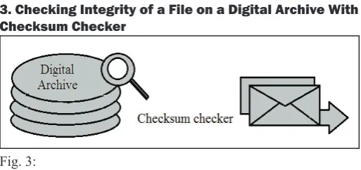
3. Checking Integrity of a File on a Digital Archive With Checksum Checker
Fig. 3:
(i). Manifest Maker
It supports transferring digital data from different sources to a digital archive.
(ii). Xena
It stands for “XML electronic normalizing for archives”. In this
file format of a digital record is determined and then converted into appropriate preservation file format based on open standards.
(iii). DPR
It stands for “Digital preservation recorder”. It records the audit information about each transfer in digital archive.
(iv). Checksum Checker
It monitors the contents of digital archive for data loss or corruption [11].
II. Problems Associated With Digital-Preservation Whenever we try to digitally preserve the data, there are many issues and problems related to it. Some of the problems associated with it are as:
The viewing problem:
• All digital formats require computer
technology to view them. We all know technology (software/ hardware/formats) move at such a rapid pace, that odds are they won’t be around when you want to view your data. This is off course unless you are viewing data right after you “preserve it” in which case, it is not really preserved now in it.
The scrambling problem:
• Data is often compressed or
“scrambled” to assist in its storage and or protect in its intellectual content. These compression and encryption algorithms are often developed by private organization that will one day cease to support them.
The inter-relation problem:
• Digital information is often
linked to other items. This is much more evident in the digital world than the physical. If these linked are not maintained, the information is incomplete, incorrect or just plain. It doesn’t make any sense at all.
The custodial problems:
• Who is the custodian of the digital
document? What if someone changes the content without telling the custodian? After all digital content is dynamic and easily changed.
The translation problem:
• If we need software to interpret
data as software changes version to version, will it be translated differently in subsequent versions [8].
A. Drawbacks of Digital Preservation
Digitally preserving the data have its own challenges associated with it. While embodying clear advantages--precise replication, machine processing, online content delivery--information in
digital form also introduces a host of difficulties with regard to
access and preservation. Some of the drawbacks are discussed below:
1. Massive Storage Failure
No matter how much money you spend on the system holding your data, there are still many ways in which it can fall over and create opportunities for data to be last. This may be from hardware/ software failure or an act of war. The longer you try to store data the more likely this will occur.
2. Bit Rot
No digital storage medium is completely reliable over a long period of time.
3. Outdated Media
Over time all kinds of digital media become outdated. Technology is driven by innovation which unfortunately leads to very short periods of relevancy before redundancy. Data stored on redundant media becomes effectively useless if the appropriate hardware is not available to read it.
4. Outdated Formats, Applications and Systems
As hardware becomes redundant, so do file formats and the software which interpret them. This is a difficult problem for long term storage and there are two common solutions. The first
is to preserve a copy of appropriate software and make it available wherever that data is stored. The second is to transfer data to an acceptable format.
5. Intentional Attacks
Some people intentionally destroy or damage digital assets for a variety of reasons. As much of the information is currently located in open access repositories accessible via the internet which makes it more vulnerable to attack.
6. Lack of resources
Some institutions do not have the resources, usually financial, to
consider digital preservation.
7. Organizational Failure
This is a massive threat to long term digital storage of any kind. Technology is so dynamic not only in innovations but also movements with vendors and competition killing off what seemed to be at one point very strong technology. For this reason it would be a folly to rely too heavily on any one vendor/system/sponsoring organization because they change and often change quickly. Digital assets which need to be preserved long term must be protected from the failure of any one organization. Unfortunately this is easily said but hard to plan for us such a dynamic environment.
8. Loss of Context
Some data can be related and this relationship can be vital to data
interpretation. Unfortunately if this information is not identified and preserved when information is first stored it is unlikely
to be ever recovered. The longer the data is kept without this relationship, the less likely it is to ever be resolved.
9. Data Compression
implementations, the extra complexity added by data compression
can increase the system’s cost and reduce the system’s efficiency,
especially in the areas of applications that require very low-power VLSI implementation [8].
III. Data Compression
Data compression is defined as the process of encoding information
using fewer bits than the original representation of the information would use. Data compression is often known as bit – rate encoding or source coding [2].
A. Importance of Compression
Data compression is very useful because it helps to reduce the consumption of expensive resources such as the hard-disk space or the transmission bandwidth.
Example: - For compressing a video we may require expensive hardware to decompress the video fast enough to be viewed as it is being decompressed. So, the data compression schemes therefore involves tradeoffs among various factors including the degree of compression, the amount of distortion to be introduced and the computational resources required to compress and to decompress the data [2].
B. Types of Compression
1. Lossless Compression Algorithm
These types of algorithms usually exploit the statistical redundancy in such a way so, as to represent the sender’s data more concisely without an error.
Example: - In word ‘BAHRA’ the letter ‘A’ is much more common than the letter ‘Z’ and the probability that the letter ‘S’ will be followed by letter ‘Z’ is very small.
2. Lossy Data Compression Algorithm
This algorithm generally works if some loss of fidelity is acceptable
in the text to be compressed.
Example: - As we know that the human eye is much more sensitive to sudden variations in luminance than it is to the variations in the color. The JPEG image compression algorithms works in part by “rounding off” some of the less important information.
3. Lossy
Lossy image compression is generally used in digital cameras, to increase the storage capacities with minimal degradation of picture quality.
4. Lossless
The Lempel-Ziv compression that is explained later is amongst the most popular algorithms for lossless storage [2].
IV. Source Modeling
We explain it with the help of an example, suppose we go to a library. This library has a large selection of books – say 100 million. Each book is very thick; say each book has 100 million characters or letters in them. When we go to this library we will in random manner select some book. This chosen book is the information source to be compressed.
Mathematically the book we selected is denoted by
X= (x1, x2, x3, x4,…………xn)
Here, ‘X’ represents the whole book, and ‘x1’ represents the first
character, ‘x2’ represents the second character and so on. As, 100 million is very large so, we assume that the characters
are just infinite in number.
In order to simplify the things, let us assume that all the characters in all the books are either a lower-case letter (‘a’ through ‘z’) or
just a‘space’. The source alphabet ‘A’ is defined to be a set of all
27 possible characters:
A = {a, b, c, d, e, f, g, h, i, j, k, l, m, n, o, p, q, r, s, t, u, v, w, x, y, z, space}
Here we need to keep one thing in mind that we do not know in advance, that which book we will select. But we know that, we are selecting a book from this library.
From, that perspective, we can say that the characters in the book (xi, i=1, 2, ……..) are random variables which take values on
the alphabet A. so, the whole book is just an infinite sequence of
random variables that is X is a random process.
V. Shannon Lossless Source Coding Theorem
It is just based on the concept of block coding. Here, we introduce a special information source in which alphabet consists of only two letters.
A = {a, b}
Letters ‘a’ and ‘b’ are both likely to occur equally.
Given that ‘a’ occurred in the previous character, the probability that ‘a’ occurs again in the present character is 0.9. Similarly we can predict for ‘b’. This is known as binary symmetric markov source’.
An nth order block code is just mapping which assigns to each block of n consecutive characters a sequence of bits of varying length.
A. First Order Block Code
Each character is mapped to single bit.
B1 P(B1) Codeword
a 0.5 0
b 0.5 1
R= 1 bit/ character.
Example: -
Original data:- aaaaaaabbbbbbbbbbbbbaaaa Compr data:- 000000011111111111110000
Here, we note that 24 bits are used to represent 24 characters. An average of 1 bit / character.
B. Second Order Block Code
Pairs of characters are mapped to one, two or three bits.
B2 P(B2) Codeword
aa 0.45 0
bb 0.45 10
ab 0.05 110
ba 0.05 111
Example:-Original data:- aa aa aa ab bb bb bb bb bb bb aa aa Compr data:- 0 0 0 110 10 10 10 10 10 10 0 0
Here we, note that only 20 bits are used to represent 24 characters an average of 0.83 bits/character.
C. Third Order Block Code
In this case triplets of characters are mapped to bit sequence of lengths one through six.
B3 P(B3) Codeword
aaa 0.405 0
bbb 0.405 10
aab 0.045 1100
abb 0.045 1101
bba 0.045 1110
baa 0.045 11110
aba 0.005 111110
bab 0.005 111111
R= 0.68 bits/ character
Example:
-Original data:- aaa aaa abb bbb bbb bbb bba aaa Cmprd data:- 0 0 1101 10 10 10 1110 0
Here, only 17 bits are used to represent 24 characters an average of 0.71 bits/character.
The rates shown in the tables are calculated from:
R= 1/n ∑p(Bn) l(Bn) bits/ sample.
Where l (Bn) is the length of the codeword for block Bn.
So, we came to know that the higher the order the lower the rate i.e. (better compression).
VI. Variable Length Code for a Given Message
In this type the code that is used to represent a character in the given message is of variable size.
Example: -
a b r
1100001 1100010 1110010
a
b
r
000
001
100
a b r
101 111 110
So, here we can see that the characters remain the same where as their code gets changed i.e. they are of variable length.
The main advantage of the variable length encoding is that it provides better compression.
VII. Huffman Algorithm
This algorithm was given by David Huffman in 1950’s
A. Huffman Encoding Algorithm is as:
-Count the frequency Ps of each symbol ‘s’ in the message.
•
Start with one node corresponding to each symbol ‘s’ with
•
frequency ps.
Repeat until a single tree is formed.
•
Select two trees with minimum weight P1 and P2. Merge
•
them into a single tree with weight P1+P2.
Applications: - JPEG, MP3, MPEG, GZIP etc.
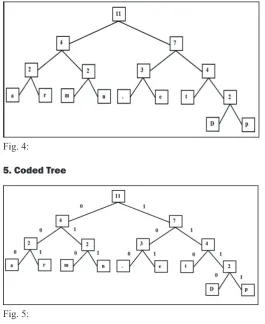
Example of Huffman coding Department.
1. Characters in this sentence are as: -{D, e, p, a, r, t, m, n, .}
All the spaces, special characters upper-case and small-case letters are treated individually.
2.
Character Frequency
D 1
e 2
p 1
a 1
r 1
t 2
m 1
n 1
. 1
3. Building a Tree:
-Create binary tree nodes with character and frequency of
•
each character.
Place nodes in a priority queue. It should be noted that
•
the lower the occurrence the higher be the priority in the queue.
Use binary tree nodes.
•
Public class huffnode {
public char mychar; public int myfrequency;
public huffnode myleft, myright; }
4. Queue after inserting all the nodes:
-D p a r m n . e t
1 1 1 1 1 1 1 2 2
While priority queue contains two or more nodes. Create new node.
•
Dequeue node and make it left subtree.
•
Dequeue next node and make it right subtree.
•
Frequency of the new node equals sum of frequency of the
•
So, after performing these steps the final tree we will get the tree
as follows:
-Fig. 4:
5. Coded Tree
Fig. 5:
6. Code Generated for Each Character
Character Code
a 000
r 001
m 010
n 011
. 100
e 101
t 110
D 1110
p 1111
So, 29 bits are used to encode the text. ASCII would take 72 bits
would be used. Also if modified code would have been used then
total number of bits used to represent this text would be (4*9) = 36.
B. Decoding the Huffman Code
1. Tree constructed for Each Text File
Consider frequency for each text file. •
Big hit on compression especially for smaller files. •
2. Tree predetermined
It is based on the statistical analysis of the text files or the •
text types.
Once receiver has the tree it scans the incoming bit-stream. 0 -> go left.
1 -> go right.
Encoded stream of bits: - 00000101001110010111011101111 Decoded data is:
a, r, m, n, ., e, t, D, p
The time complexity of the Huffman’s algorithm is O(n log n). using a heap to store the weight of each tree, each iteration requires O(log n) time to determine the cheapest weight and insert the new weight. There are O(n) iterations, one for each item.
VIII. Fixed Length Code for a Given Message
In this type the code that is used to represent a character in the
given message is of fixed size.
a b r
0000 0101 1000
a b R
1111 0111 1010
IX. Lempel-Ziv-Welch Algorithm for Data Compression
When encoding a byte stream,the first 28 = 256 entries of the
string table, numbered 0 to 255, are initialized to hold all the
possible one-byte sequences. The other entrieswill be filled in as
the message byte stream is processed.
Create a symbol table associating a fixed length codeword •
with some previous substring.
When input matches string in symbol table, output associated
•
codeword.
Length of strings in symbol table grows hence
•
compression.
A. LZW Compression Algorithm STRING = get input character
•
WHILE there are still input characters DO
•
CHARACTER = get input character
•
IF STRING+CHARACTER is in the string table then
•
STRING = STRING+character
•
ELSE
•
Output the code for STRING
•
Add STRING+CHARACTER to the string table
•
STRING = CHARACTER
•
END of IF
•
END of WHILE
•
Output the code for STRING
•
Example
Now, let’s suppose our input stream we wish to compress is “banana”, and that we are only using the initial dictionary:
Index Entry
0 a
1 b
2 d
Now the encoding steps would proceed like this:
So, 16 digits are used to encode the text. ASCII would take 48 bits.
Also if modified code would have been used then total number of
bits used to represent this text would be (4*6) = 24.
B. LZW Decompression Algorithm: Read OLD_CODE
•
output OLD_CODE
•
WHILE there are still input character
•
DO
•
Read NEW_CODE
•
STRING = get translation of NEW_CODEoutput STRING
•
CHARACTER = first character in STRINGadd OLD_CODE •
+ CHARACTER to the translation table OLD_CODE = NEW_CODE
•
END of WHILE
•
Now we will decode the string we have just encoded rather compressed.
Applications of LZW algorithm: GIF image format, TIFF and
PDF files.
Uses of LZW algorithm: LZW compression became the first
widely used universal data compression method on computers.
A large English text file can be compressed through LZW to obtain
half its original size.
Time complexity of LZW algorithm: The time complexity of LZW algorithm is same as that of the Huffman’s algorithm i.e. O(n log n).
X. Conclusion
As both the Huffman and LZW algorithm are having the same time complexity, and both are used to compress and decompress
the files. so, depending upon the file type to be compressed first
algorithm is considered superior to other in some cases, where as in other cases the second algorithm is considered better than
the first.
So, given below a chart of compression ratio for different file
types of both Huffman and LZW algorithm.
File Type Compression/ratioHuffman algo. Compression ratio/ LZW
.doc 45 – 76 % 38 – 88 %
.bmp 73 – 81 % 68 – 93 %
.gif -9 % -43 %
.jpg -1 – -5 % -16 - -41 %
Reference: “Comparative Study between Various Algorithms of Data Compression Techniques”
From the chart above we can make the following conclusions: LZW and Huffman give nearly results when used for
•
compressing document or text files, as appears in the table.
The difference in the compression ratio is related to the different mechanisms of both in the compression process; which depends in LZW on replacing strings of characters with single codes, where in Huffmandepends on representing individual characters with bitsequences.
When LZW and Huffman are used to compress a binary file, •
LZW gives a better compression ratio than Huffman.
When LZW or Huffman is used to compress a file of type •
gif or type jpg, the compressed file size is larger than the original file size; this is due to being the images of these files
are already compressed, so when compressed using LZW the number of the new output codes will increase, resulting
in a file size larger than the original , while in Huffman the
size of the binary tree built increases because of the less of probabilities, resulting in longer bit sequence that represent
the individual dots of the image, so the compressed file size
will be larger than the original . But because of being the new output code in LZW represented by 9 bits, while in Huffman the individual dot is represented with bits less than 9, this
makes the resulting file size after compression in LZW larger
than that in Huffman [1].
References
[1] Mohammed Al-laham, Ibrahiem M.M. El Emary, “Comparative Study between Various Algorithms of Data Compression Techniques”, Faculty of Engineering, Al Ahliyya Amman University, Amman, Jordan, 2011. [2] M. Burrows, D.J. Wheeler,“A Block-sorting Lossless Data
Compression Algorithm”, Digital Systems Research Center 130 Lytton AvenuePalo Alto, California, 2011.
[3] Guy E. Blelloch (2010),“Introduction to Data Compression”, Computer Science Department Carnegie Mellon University blellochcs.cmu.edu. 2011.
[5] Richard Fyffe, Deborah Ludwig, Beth Forrest Warner, (2005),“Digital Preservation A campus wide perspective”, 2011.
[6] R.P Brent,“A linear algorithm for data compression”, 2011.
[7] “Long Term File System (LTFS): An OpenFormat
Specification for LTO 5 and Onwards”, Centre of excellence
for digital preservation. Sponsored by ministry of information technology “Government of India”. 2011.
[8] “A state of digital preservation an International perspective”, (2002) Conference Proceedings Documentation Abstracts, INC. Institutes for Information Science WASHINGTON, D.C., 2011.
[9] Dr. Ramesh C Gaur,“Digitization and Digital Preservation of Indian Cultural Heritage”, Multimedia Digital Library Initiatives at IGNCA, New Delhi, 2011.
[10] National Workshop on,“Digital Preservation in India”, held on November 7, 2008 at Federation of Indian Chambers of Commerce and Industry (FICCI), Tansen Marg New Delhi, 2011.
[11] “Dissecting the digital preservation in software platform”, 2011.
[12] (2011) [Online] Available: http://www.cs.auckland.ac.nz/ software/AlgAnim/huffman.html
[13] (2011) [Online] Available: http://www.cs.auckland.ac.nz/ software/AlgAnim/lzw.html
[14] (2011) [Online] Available: http://www.wikipedia.com [15] (2011) [Online] Available: http://www.cdac.in
[16] (2011) [Online] Available: http://www.trustlto.com/LTFS_ Format_To%20Print.pdf
[17] (2011) [Online] Available: http://www.lto-technology.com/ About/faq.html
[18] (2011) [Online] Available: http://sysdoc.doors.ch/
SEAGATE/LTO%20Ultrium%20Confirming%20Value%20