Modification of Internal Representations as a Mechanism for Learning in Neural Systems

Modification of Internal Representations as a Mechanism for

Learning in Neural Systems

Ken Kangda Wren

University College London

A dissertation submitted for the degree of Doctor of Philosophy at Physiology Department UCL. London University

ProQuest Number: U641981

All rights reserved

INFORMATION TO ALL USERS

The quality of this reproduction is dependent upon the quality of the copy submitted. In the unlikely event that the author did not send a complete manuscript and there are missing pages, these will be noted. Also, if material had to be removed,

a note will indicate the deletion.

uest.

ProQuest U641981

Published by ProQuest LLC(2015). Copyright of the Dissertation is held by the Author. All rights reserved.

This work is protected against unauthorized copying under Title 17, United States Code. Microform Edition © ProQuest LLC.

ProQuest LLC

789 East Eisenhower Parkway P.O. Box 1346

D e d ic a te d t o my p a r e n t s

and L aura,

Declaration:

This project has been carried out under the supervision of Dr. A. R. Gardner-Medwin, whose original idea prompted this research. Except where explicit reference is made, the material contained in this dissertation is the result o f my independent research, and is, to the best of my knowledge, original.

Ackn owledgement

Description of Thesis

Title: Modification of Internal Representations as a Mechanism for Learning in

Neural Systems.

1. Incoming sensory signals are processed by hierarchically organised modules in the brain. In certain contexts, this may be modelled by a feedforward layered network of interconnected binary units. The activity patterns in the intermediate layers are internal representations.

2. A new learning algorithm uses projections from the desired output to modify internal representations. Biologically realistic 2-layer synaptic rules can then be applied to cause the associated input to evoke the modified representation(s) that are more readily trained to produce the target output.

3. Simulation is carried out on benchmark tasks for 3-layer feedforward networks. Comparisons with other popular algorithms are made. The results suggest that the new algorithm has better generalisation performance with faster or equal learning speed on the tasks simulated.

4. The learning algorithm is generalised to a multi-layer network setting, in which internal representations are dynamically constructed.

CHAPTER 1 INTRODUCTION...1

Section 1.1 Biological Basis of Standard Network M odels... 2

Section 1.2 Standard Network Formalism: The Weight-Centric Approach... 3

Section 1.3 An Alternative Proposal: The Pattern-Centric Approach...4

Section 1.4 Relationship to Broader Theoretical Issues...7

CHAPTER 2 BIOLOGICAL BACKGROUND... 9

Section 2.1 Neurons...9

2.1.1 Membrane Potentials... 9

2.1.2 The Frequency C ode... 11

2.1.3 Synapses...13

2.1.4 Synaptic Integration and Plasticity... 15

Section 2.2 Basic Characteristics of the Cortex...17

2.2.1 Cortical Layering and Columnar Organisations...17

2.2.2 Localization of Cortical Functions... 18

CHAPTER 3 NEURAL NETWORK MODELS...21

Section 3.1 Rosenblatt’s Simple Perceptron... 21

3.1.1 The Basic Architecture...21

3.1.2 The Learning Procedure...22

3.1.3 Limitations... 25

Section 3.2 Multi-layer Perceptrons... 25

3.2.1 Pattern-Centric vs. Weight-Centric Learning Strategies... 26

3.2.2 The Standard Gradient-Descent Algorithm...27

Section 3.3 Self-Organising Networks... 32

3.3.1 Supervised and Unsupervised Learning... 32

3.3.2 Competitive Learning Strategy... 33

3.3.3 Kohonen N etw ork... 34

Section 3.4 Homogeneous and Hierarchically Organised Attractor Networks... 35

3.4.1 Autoassociative Attractor Networks...35

3.4.2 Hierarchically Organised Attractor Networks...37

CHAPTER 4 THEORETICAL ASPECTS OF THE RA ALGORITHM... 40

Section 4.1 An Overview of the RA Algorithm...40

4.1.1 Fundamental Steps in the RA Algorithm... 40

4.1.2 The Key Elements and the Biological Plausibility of R A ... 41

Section 4.2 Modification of Internal Representations via Reverse Connections in RA... 48

4.2.1 The Basis for Constructing Internal Representations...49

4.2.2 Constructing a Modified Representation... 54

4.2.3 Setting the Number of Cells in a Representation...56

4.2.4 Random Tuning of Reverse Activation Strength...59

Section 4.3 The Reverse Weight M atrix... 60

4.3.1 Identification o f the Ideal Reverse Weight M atrix... 61

4.3.2 Standard Inverse Problems: Inverse Optics, Inverse M odels... 63

4.3.3 The Transpose as a Possible Inverse Operator... 66

4.3.4 Weight Statistics, Activity Ratios and Inversion by Transpose... 67

4.3.5 Comments on Initial Weight Statistics and Activity Ratio Setting for RA learning 77 Section 4.4 Reverse Activation Algorithm in Multi-layer Networks... 78

4.4.1 Using Stationary States to Constmct Internal Representations... 79

4.4.2 Proof that Stationary States Always Exist on the Given Network...80

4.4.3 Interpretation of Generalised R A ... 82

CHAPTER 5 SIMULATION OF REVERSE ACTIVATION ALGORITHM....83

Section 5.1 Methodology... 83

5.1.1 Sampling Tuneable Parameters...84

5.1.2 Preparations o f Initial Conditions... 89

Section 5.2 Data for Two Benchmark Learning T asks...90

5.2.1 CT Discrimination Task... 90

5.2.2 Mirror Symmetry Discrimination T ask... 105

CHAPTER 6 DISCUSSION AND CONCLUSIONS... 119

Section 6.1 Optimal Activity Ratios... 119

Section 6.2 Random Tuning of Reverse Activation Strengths... 121

6.2.1 Purposeful Random Fluctuation...121

6.2.2 Applying a Population search Algorithm...124

Section 6.3 Generalisation Performance...125

Section 6.4 Technical Questions That Require Further Investigations...125

6.4.1 Comparisons between Variants of BP and RA... 125

6.4.2 Simple and Complex Outputs... 127

Section 6.5 Efficient Sensory Processing and Representation... 125

6.5.1 The Goal of Sensory Information Processing... 128

6.5.2 Different Concepts of Redundancy Reduction... 128

6.5.3 Investigating Sparseness in the RA Context...130

Chapter 1 Introduction

The study seeks to gain insights into sensory representation and learning mechanisms in the brain with the aid of computer simulation of networks o f artificial neurons. A new learning algorithm for a certain class of networks will be proposed and investigated.

This chapter introduces a novel approach to thinking about learning, which underlies most o f the investigations in the thesis. Learning, in most models, including those considered here, is assumed to be brought about by changes in synaptic weights. But the effects of learning are more usually discussed in terms o f the resultant internal representations (i.e. the patterns o f cellular activity that arise from the stimuli), and how these representations relate to the learning objective. This perspective can be constructive simply because the activity patterns are readily observable variables, more so than weight changes. The starting point of this thesis is the suggestion that explicit changes of internal representations, with the objective of achieving representations that make learning easier, may in fact be built into a learning algorithm.

After this general approach has been set out, a review of both relevant biological issues and related theoretical approaches will follow, before the RA algorithm is analysed with both theory and simulations.

Section 1.1

Biological Basis of Standard Network Models

The term neuron is used repeatedly in the thesis to refer to abstract neurons used in artificial network models. A biological neuron has more complex behaviours than the stereotypical abstract neuron. Radically different types of neurons exist in the brain. Further, each of the brain’s regions is a vast network o f distinctive sub-networks of neurons. In contrast to this complexity, most network models have a simple architecture consisting of identical units that are essentially summation devices coupled with a transfer function. Despite these differences, there are many reasons for accepting such networks as relevant to the study of the brain.

but there is seldom good reason to think that what it can achieve could not be achieved by real neurons, nor vice versa - that what it cannot achieve could be achieved by real neurons.

At an appropriate scale, the organisation of neurons in the brain is fairly uniform. The same simple architecture found in one locality (e.g. the retina) may appear elsewhere also (e.g. the olfactory bulb) (Shepherd, 1974). Further, perhaps more importantly, in many parts of the brain (e.g. association areas o f neocortex), the architecture seems to be governed by simple rules, with large numbers o f neurons or functional groups of neurons forming connections specified largely by global conditions such as layering, and of cell and synaptic densities. The study of simple networks seems likely to be important for the understanding of local functions, as well as large scale organisation in the brain.

Section 1.2

Standard Network Formalism: The

Weight-Centric Approach

Most artificial networks, be it recurrent or feedforward, are pattern associators: they associate an output activity pattern to an input activity pattern by way of system dynamics as determined by the architecture and the weights o f connections. They are particularly useful in understanding associative memory and feature detection in sensory pathways. To focus the argument, let us concentrate on multi-layered feedforward networks.

learning involves iteratively changing each weight according to its effect on the performance function for the purpose of optimisation. Learning and generalisation are thus reduced to interpolation and extrapolation: the network represents a particular model (in the sense used for Statistical Inference), where the weights are the adjustable parameters. Any such learning algorithm is a way of computing the ‘best fit’ parameters. Weights are the fundamental variables in this formalism, while activity patterns (on intermediate layers) are somewhat incidental; that is, such learning models lose nothing if the significance of these patterns is completely disregarded. However, these activity patterns attract great interest because they correspond (or at least the individual elements of them do) to the most important observable in neurophysiological studies.

This approach gives a simple mathematical formalism to the learning problem, and leads to many different learning algorithms, the most popular of which is Back- Propagation (BP). One disadvantage of the approach, apart from being a rather rigid view of learning, is that most of the derived algorithms, such as BP, are not biologically plausible (see Section 3.2.2). Further, it is unsatisfactory that representational patterns, despite being a primary variable in neural science studies, are peripheral in these models of learning.

Section 1.3

An Alternative Proposal: The Pattern-Centric

Approach

representations (defined as the activity patterns on the intermediate layers). Weight

changes are still the intermediary, but they are driven by the goal o f achieving a chosen modified representation via local Hebbian type synaptic rules. The key question is what constitutes an improved internal representation.

In the context o f feedforward networks, the ideal representation for a novel input would be one that leads, with no weight changes, to the generation o f appropriate outputs. Novel inputs are only likely to produce such ideal representations if there is a remarkable correspondence between the information processing in a network and the characteristics o f the world that govern what are appropriate outputs for particular input patterns. More realistically, the existing representation o f a novel input will not be ideal, but may be improved by altering the input processing so that fewer weight changes are required between representation and output in order to generate appropriate patterns.

easily learn to generate the correct output. Several questions arise and will be addressed: can the suggestion be analysed theoretically; to what extent could it benefit learning; and how can the necessary conditions be arranged?

There have been earlier attempts at a pattern-centric approach, particularly the so- called CHIR ("choosing internal representations") (Grossman et. al. 1988; Grossman, 1989; Nabatovsky et. al. 1990; Abramson et. al. 1993); also see (Domany et. al. 1995). These proposals rely on active search in a vast table o f potential internal representation patterns. Some other versions of CHIR (Rujan, Machand, 1989; Mezard, Nadal, 1989) take a more explicitly geometric approach, which still amounts to a ‘home-in’ mechanism in the high dimensional representation space in order to determine the ‘appropriate’ representations. Further, the final number of hidden units and hidden layers in the solution found is uncertain, and there is no guarantee that the trivial solution (i.e. one exclusive hidden unit for each input-output pair) would not emerge, see (Domany et. al. 1995) for instance.

Unlike the above CHIR’s, the RA algorithm does not rely on a time-consuming explicit search in the representation space. Instead, it iteratively modifies existing representations via biological mechanisms. The weight-based algorithms such as BP also iteratively modify internal representations, but only as a by-product o f weight modification. The important difference in RA is that weight changes are driven by changes in internal representations, while in BP the exact opposite happens.

parameter tuning. The result shows that on tasks tested, the RA algorithm has better learning speed and generalisation performance. The latter is consistent with known theories on generalisation. It will be argued that the very mechanism for improving internal representations in the RA algorithm promotes better generalisation performance. RA is outlined and studied in Chapter 4, 5 and 6. A population search technique may be applied to the RA algorithm to improve its practicality, as discussed in Chapter 6.

Section 1.4

Relationship to Broader Theoretical Issues

The pattern-centric approach to learning is readily related to broader issues in the study of the brain. Crudely speaking, the subject of information processing in the brain can be studied at the system level or at the neural (network) level. The former concerns overall characteristics and complex functions of the brain, and offers explanations in terms of information and computational theories. The latter concerns the implementation or the manifestation of system level theories in terms of computational algorithms that can be justifiably described as being ‘neural-network’, based on known biological and physiological evidence. A complete understanding requires comprehension at both levels. Ideally, one formulates computational theories, which then can be seen at work in a neural network context; conversely, one can hope that a particular discovery at the neural network level has a certain higher level rationale.

provides an arena for studying the effect of sparseness on learning in feedforward networks o f more than 2 layers.

The RA algorithm implicitly requires a short-term memory for paired patterns, independent o f the representational changes that will eventually be brought about, contributing to long term memory. It therefore touches on the issue of memory consolidation in the brain. Temporal storage is required for at least the most recent activity patterns on each layer so that conditions can be set up for creating and learning the improved representations. Quite different mechanisms, possibly in different sites, may be involved as an intermediate step to the consolidation o f the long-term memory, which could be modelled as the inter-layer weights. Both high quality transient memory and the ability to re-generate patterns of activity without related sensory stimuli (in imagination, rehearsal, dreams, etc.) are in fact prominent features of the nervous system, whose functional role is not clear. This adds to the plausibility and interest of the mechanisms o f the algorithm.

Chapter 2 Biological Background

It is helpful to review the biological reality behind the theoretical speculation ahead, for motivation, context and perspective. The chapter may be skipped by readers familiar with the subject. Section 2.1.1, 2.1.3, 2.1.4 and Section 2.2.1 contain standard facts/theories based mainly on Shepherd (1974) and Nicholls, Martin, Wallace (1992).

Section 2.1 Neurons

2,1.1 Membrane Potentials

Most neuronal behaviours stem from the selectivity properties o f channels on the cell membrane. Some channels may be open only to cations, some to anions. While most anion channels are non-specific, cation channels may be specific to, for instance, potassium, sodium or calcium. Ionic channels are usually gated. The selectivity and gate mechanisms are responsible for the electrical signals generated within the nervous system. Various mechanisms can cause ion channels to change states thereby disturbing the established equilibrium and pushing the membrane away from its resting state. Some channels respond to chemical signals such as neurotransmitters, some to membrane deformations due to mechanical forces, and still others to the membrane potential itself. These mechanisms provide the means through which neurons respond to stimuli and each other.

dynamic. Sodium action potentials, stereotyped cycles of rapid membrane depolarisation and repolarisation lasting up to 2 milliseconds, result from the properties of voltage gated Na+ and K+ channels and occur in an all-or-nothing fashion.

If a depolarising potential raises the local membrane potential sufficiently, the sodium channels on that patch will open rapidly, but transiently. The increase will cause a sudden influx o f Na^ ions since sodium is much less concentrated inside the cell. The local membrane potential then will shoot up to typically +40mV within 0.5-1 millisecond. Potassium permeability also responds to increase in membrane potential, though its reaction is slower but more persistent, lasting several milliseconds. The resulting persistent outgoing potassium current will drive the membrane potential rapidly down, even to below the resting potential for a time, causing the so-called refractory period, before the resting potential is restored, thus completing the cycle, known as an action potential.

2,1,2 The Frequency Code

Because the action potential is all-or-nothing and self-reproducing through the use of local energy stores, it provides the basic means of long distance communication in a biochemical environment, where reliable communications via passive flow of analogue electrical signals are possible only on a scale measured in tens of micrometers.

Since the action potential generated down an axon is exactly the same as the original action potential, there is no transmission loss. However the all-or-nothing dependence of action potential on stimuli also means that no information is conveyed in the time course (‘shape’) of the potential. It is the event itself, or more precisely, the number of action potentials in a given period, which carries information. This is called frequency coding.

Given the time scale o f an action potential of the order of 1 millisecond, one may divide time into 1 millisecond intervals so that there is either 1 action potential generated or none. The frequency code can therefore be represented as a sequence of 1 and O’s. The upper limit of transmission rate is around 1000 bits/second. However, neurons on average fire less than half of the time, and there is correlation between firing intervals. These redundancies alone place the upper limit at about 500 bits/second. One may expect further redundancies implemented in order to counter noise.

mammalian lateral geniculate neurons indicates a rate no more than 30 bits/second (Tovee et. a l, 1993).

The above approach is not adequate for studying information processing in the cortex. Each cortical neuron can receive signals directly from as many as 10^ other neurons, only a small fraction o f which are sensory afferent signals. It is seldom clear exactly what information is conveyed to and by a particular neuron, and information about most aspects o f sensory stimuli are probably conveyed in a population code, spread across many neurons.

There is perhaps a deeper reason why cortical neurons must be analysed differently. Cortical neurons are not merely encoders that transmit information: there is no homunculus waiting to analyse the information. The population of cortical neurons as a whole is in some sense the ‘end-user’ of sensory information. The point o f interest is not so much how a neuron encodes the incoming information and passes it on, but how it responds to the incoming information (relayed to it by lower level neurons). If one accepts that mental activity is a collective phenomenon made up by the individual responses of cortical neurons, then the activity pattern across cortical cell populations becomes a primary concern in this context. Thus, as one moves into the cortex, one stops focusing on the details of the frequency code adopted by an individual neuron, but on how sensory information is represented by the activity patterns of cell populations; the concept o f ‘population code’ or ‘internal representation’ becomes the theme. We shall address these issues further in Section 2.2 and 2.3.

2.1.3 Synapses

The states of ionic channels on the cell membrane, and therefore the membrane potential, can be altered via a variety of mechanisms. Sensory neurons respond to direct mechanical (pressure) and physical (light, odour) stimulation. Most neurons including sensory neurons also receive direct electrochemical stimuli from other neurons, so that signals can be passed on, enhanced, modulated, and transformed from neuron to neuron. A synapse is a physical point o f contact through which such interactions take place. At a synaptic site, the gap between the membranes of two cells ranges from 20-300 Angstrom, or 2-30 nanometers across, depending on the nature of the synapse. By far the most common and more sophisticated synapses are chemical synapses. They are strongly directional. The postsynaptic cell can act on the presynaptic cell via the same synapse but generally not in the same manner as the forward action.

Chemical synapses rely on neurotransmitters to change the postsynaptic membrane potential. It takes time however for vesicles, little parcels o f neurotransmitters, to be released, to diffuse across the synaptic cleft, and to take effect. The delay between the pre- and post-synaptic potential is typically 0.5 to 1 millisecond. O f the delay, only about one-tenth can be accounted for by diffusion. The rest of the Tong’ interval is mainly due to the fact that to release the vesicles. Calcium must be present. It has been found that the direct effect of the presynaptic potential is mainly the opening of Ca^^ channels, through which extracellular Ca^^ ions flow inwardly.

total PSP depends on the number of quanta released. The probability o f a quantum being released upon the arrival of a presynaptic potential is constant; each release is typically statistically independent. These assumptions explain the observed statistics of fluctuations in postsynaptic potentials very well.

One striking fact o f the vertebrate nervous system is that the mean number of quanta released per presynaptic impulse by synapses in the central nervous system can be as much as 300 times lower than those in the periphery (such as neuromuscular junctions). However, the probability of release per presynaptic impulse can be as high as 0.9 in the central system. This dramatic difference in the mean quantal content is merely an indication that the central nervous system is concerned with the integration of information so that no one synapse has a dominant effect.

Once arrived at the postsynaptic membrane, some neurotransmitters act by directly activating appropriate ion channels. Many transmitters act by indirect mechanisms: they combine with receptors that are not ion channels themselves. The resulting substance then either is acted upon by other intracellular messengers, or acts directly, to modify the activity o f other receptors, ion channels or ion pumps, thereby changing the membrane potential. Indirect synapses are usually slower.

2.L 4 Synaptic Integration and Plasticity

A cortical neuron can receive as many as 10"^ convergent synapses. The effect of an individual synapse is rarely enough on its own to generate aetion potentials in the postsynaptic cell. The overall activity of the postsynaptic cell is the result of the interplay between inputs from many convergent synapses.

The efficacy or strength of a (chemical) synapse usually refers to the size of the resulting post-synaptic potential (PSP) and the length o f synaptie delay, for a given ‘amount’ o f presynaptic stimulation. Efficacy can vary both in the short term and in the long term. These variations can be due to either pre- or post-synaptic mechanisms. By altering the efficacy of synapses, a neuronal system may be able to learn.

It is tempting to assume that the PSPs of all synapses are integrated by a simple numerical summation, and that the efficacy of a synapse, which is modifiable, can be seen as the weighting factors in the sum; as the system leams, these ‘weights’ will be modified in some way as a result of repeated pre- and post-synaptic activities. This is, broadly speaking, what standard artificial neural network theory assumes, partly because other alternatives are difficult to handle. This simplified picture o f neuronal eomputation is used extensively in network modelling (diseussed in Chapter 3). Presently, let us compare this pieture with the eurrent knowledge o f biological synaptic integration and plasticity.

well-timed inhibitory PSP (EPSP) further down the axon/dendrite can kill off an excitatory PSP (EPSP) very effectively. In addition, even at a single synaptic site, repetitive stimulation may enhance PSPs by virtue of temporal integration, with each PSPs adding to the falling phase of the one before; this happens when the frequency of stimulation is high enough (which is possible since PSPs have a much longer time course than action potentials).

Is the plasticity o f synapses any simpler to capture in modelling? Experimental evidence does support the basic idea that synaptic strength can be modified. In invertebrates (Leech and Aplysia), short-term and long-term synaptic changes have been extensively studied, and can directly account for modifications in the animal’s behaviour. However, the detailed modification prescriptions in various learning models such as those introduced in Section 3.2 are difficult if at all possible to verify.

One can see clearly from the above that plasticity is a complex phenomenon that involves a long sequence of biochemical events. As such, it lends itself to regulation by many potential mechanisms. There is increasing evidence that indeed even the plasticity of a synapse is regulated. This is termed as metaplasticity, that is, a modification o f the synapse that manifests itself not as a change in the synaptic efficacy, but as the change in the ability of the synapse to change its efficacy (Fischer et. al., 1997). The biological utility of metaplasticity is intuitively appealing (locking and unlocking of memory storage capacity for instance).

To conclude our brief review, while there is sufficient evidence to show that synaptic integration and plasticity do not conform to the simple form assumed in many network models, present evidence does suggest that biological synaptic integration and plasticity tend to be more sophisticated and thus potentially more powerful.

Section 2.2 Basic Characteristics of the Cortex

2.2.1 Cortical Layering and Columnar Organisations

The neocortex has six layers, compared to the three layers o f archicortex and the four to five layers o f paleocortex. The grey matter of the cortex, where most neuronal cell bodies lie, is about 2 mm thick, and covers the entire cortical surface. Wrapped inside is the white matter, which contains mostly fibres between cortical regions and glial cells. Sensory and subcortical efferent and afferent fibres are a small fraction of all the fibres in white matter. The input and output fibres enter and leave any cortical region through the depths.

layer. The contrast between the perpendicular and horizontal organisation is striking. In the perpendicular direction, the cortex is highly organised into layers; each layer is characterised by its cell and fibre content. Horizontally, i.e. within each layer, neurons and fibres are distributed more or less isotropically and homogeneously.

By columnar organisation one refers to the fact that neurons along a line perpendicular to the cortical surface have similar receptive field and response properties. In other words, they appear to be involved in the processing o f the same bits o f input signals. Physiological and anatomical evidence both put the diameter of such columns at 30- 500 micrometers. Neighbouring columns are sharply demarcated from each other: they either have distinct receptive fields or have different response properties (e.g. responding to blue rather than red; responding to tactile signals rather than auditory). However, connections between neighbouring columns appear to be rather non-specific compared to vertical connections within a column. Available evidence supports the idea that the activation of one column has a non-specific inhibitory effect on the neurons in nearby columns but a small non-specific excitatory effect on those further on; this is particularly true for pyramidal cells. This fact has inspired the winner- takes-all coding strategy, which has many interesting applications; see Section 3.3.

2.2.2 Localization o f Cortical Functions

The properties of neurons in each functionally uniform area are spatially ordered as well (Shepherd, 1974) (Nicholls, Martin, Wallace, 1992). For example, in the area 1 of somotosensory SI cortex, which receives tactile information, the receptive field o f a neuron varies systematically with its position on the surface of the cortex so that the cortical surface contains a topographical map of the body. Such a map can be found also in areas o f motor cortex. Similarly, topographical maps o f visual scene are found in the visual cortex, and tonographical maps in auditory cortex.

On the one hand, all cortical areas have the same basic cell compositions, the same basic ‘circuitry’}, and the same coding strategy (i.e. topographical representation) but on the other hand different areas of the cortex specialise to perform different functions. The inevitable questions are why and how.

It is relatively easy to explain how localisation is implemented. To obtain sensory information of different modalities, different physical/chemical processes must be utilised. For instance, sensory neurons that detect pressure are very different from those that detect odour. Hence at the detection level, the nervous system must have ‘localisation’. Functional specialisation in the cortex thus might be seen as a simple consequence of physical/chemical necessity, and would be a direct result o f well- designed carefully-specified sensory innervation. The sensory innervation argument however cannot account for the sharp demarcation observed between the receptive fields of neighbouring cortical columns, the basis o f topographical maps. It has been demonstrated instead (Kohonen, 1990) that lateral inhibition can achieve topographical maps even when each neuron receives exactly the same inputs; cf. Section 3.3.

Chapter 3 Neural Network Models

Artificial neural network models attempt to incorporate some o f the above qualitative biological characteristics of neurons and their interactions into quantitative terms so as to carry out more concrete investigations. Inevitable in this process some biological realism must be sacrificed in order to draw upon useful mathematical tools. The validity of this trade off is ultimately justified or refuted by the results.

In what follows, we shall deal with networks of simple formal neurons (see e.g. Amit, 1989). They are based on two basic assumptions: 1) sub-threshold excitations lead to no activity; and 2) at any instant, a neuron receives an input that is the linear sum o f all inputs from individual input synapses; the weights in the summation correspond to the efficacy of each of the modifiable input-synapses.

Section 3.1 Rosenblatt’s Simple Perceptron

5,

1.1 The Basic Architecture

The most basic network of formal neurons consists o f binary units arranged in two layers: the input (I) and the output (O) layer. Most concepts in neural networks are best illustrated in this simple context. The matrix Wio of modifiable weights specifies the connection strengths from a cell in I to a cell in O layer so that given input pattern

Pi, the activation Aq to output cell O i is given by

The activity of the cell Oi is binarised according to

0 ( A o ( i ) - 8 ( i) )

where 0 is a step-function, and 6 is a modifiable threshold. Note that this threshold can be absorbed. Since

A o(i)-0 (i)= Zj Wio (i ,j)Pi(j)-8 (0 =Zj’ W ’iq ( i , j ’)P’iO’),

where W ’iq is Wio with -0 (i) listed as an additional column, and where P ’l has an additional unit that is 1 (i.e. always ‘on’). Such individually adjustable thresholds will not be explicitly mentioned from now on.

The above network is able to associate an output pattern with a given input pattern. The detailed relation depends on the status of the forward weights.

3,1.2 The Learning Procedure

on, until no modification takes place, i.e. until all mappings are achieved. Learning time is measured by the number of epochs required. Most neural networks and learning algorithms follow the above training procedure.

The perceptron synaptic rule is a particular way of calculating the necessary weight modifications. It can be derived from performing gradient descent on the mean-square error-surface over all mappings in the training set. According to this rule, the change AW(i, j) to weight W(i, j) is given by the following

A W ( i J ) = X ( O V O i ) I j , (E q.3.1)

where O^i is the target output activity at cell i, Oj is the current output activity at cell i evoked by the input, and Ij is the activity of the input cell j in the input pattern, and X is some positive constant called step-size, small compared to the size o f the weights. Note that the step-size is the quantum of weight change in the binary setting and is also referred to as the learning rate.

There is a legitimate concern over whether the above synaptic rule is biologically plausible, particularly regarding the availability o f error signals (O^i - Oi) at the presynaptic sites. Gardner-Medwin suggested (in private correspondence) one way of interpreting the rule (Eq. 3.1). Note the prescribed modification, AW(i, j)= X (O^j -Oi)Ij, can be separated into two stages: one of anti-learning i.e. forgetting while the internally generated output is on, as suggested by the term -lOilj , and one of positive

evidence of the existence of anti-Hebbian synaptic modification see for example (Bell et. a l, 1990).

In the perceptron algorithm, there are 3 principle options for when a computed weight modification may be implemented. The two most commonly used methods are on-line updating and batch updating.

In the former, each weight is updated according to a prescribed formula (such as Eq. 3.1) immediately following the presentation of each pattern in training set. In the latter, the training set patterns are learned as a whole: each weight is updated only after all the input-output pairs are presented, and the modification is given by the sum of all the required modification calculated from individual patterns. The third less well- known updating procedure, proposed and referred to here as ‘total-on-line’ for convenience, is a training procedure in which individual pairings in the training set are learned completely, one at a time: weights are modified iteratively till the latest input- output mapping is learned perfectly before the next input-output mapping is presented. This ‘perfect learning’ is of course at the expense of possibly damaging the mappings already ‘perfectly’ learned before the presentation of the latest mapping.

There are subtle differences between these three methods (Finoff 94; Hassoun, 1995; Ripley 96; Saad, Solla, 1996). Briefly, the on-line method is the most volatile and sensitive to step-size. The total-on-line method can be the most stable with respect to step-size. The batch method is somewhere in between in this respect, and it is also most mathematically sound but least biologically plausible. These will be explained in more details. For small 2-layer perceptrons, such distinctions are less important as far as performance is concerned.

converge to a solution with the Pereceptron synaptic rule. The convergence of the batch procedure is guaranteed by gradient descent (to be discussed shortly).

3.1,3 Limitations

A well-known point about the simple perceptron is that it cannot learn any set of mappings that are not linearly separable (Minsky, Papert, 1969). Notice that each output unit classifies the input patterns into two categories: those that turn it on, and those that do not. Input patterns can be represented as points in a vector space, in fact, as the comers o f a hyper-cube. The above categorisation is geometrically represented by a plane separating the two sets of ‘comers’. This plane is in fact parameterised by the weights onto the output unit concemed. If the mapping problem is such that the implied categorisation by an output unit is not achievable by any plane, then it is not linearly separable. Since no planes means no solution weights, the simple perceptron cannot leam such a problem.

Section 3.2 Multi-layer Perceptrons

To resolve the above problem, extra layers of units can be introduced between the input and output layer. Typically, 3-layer networks are studied, which with a sufficiently large number of intermediate cells can leam any well-defined binary mapping, if necessary by employing cells that individually detect specific input pattems. Additional intemal layers usually do not enhance the computational capabilities, though they may permit an economy of cells.

Consider a network o f 3 layers, the input layer (I), the hidden layer (H), and the output layer (O), with numbers of binary cells (in the 0-1 representation) equal to Ni, Nh, Nq

binary pattem a binarisation operation for short. This may involve thresholds that are either fixed or, for example, adjusted to achieve a particular number of active cells. All input cells project to all hidden cells, which in turn project to all output cells. Call

the I=>H weight matrix W i h , and the H=>0 weight matrix W h o - The pattems on the H

layer are referred to as internal representations.

3,2,1 Pattern-Centric vs, Weight-Centric Learning Strategies

There are two ways to extend the basic perceptron teaming procedure from 2-layer networks to 3-layer networks. The pattem-centric way is to devise an algorithm that establishes a pattem Ph* on the H layer that is desirable as a new intemal representation and to apply the perceptron mle to Wih directly so that input pattem ?i

comes to evoke ?h* instead of its initial representation ?h. The weight changes are divided so as to achieve two new mappings: Pi=>?h* and PH*=>Po, where Pq is the target output pattem. The perceptron mle can be applied at each stage. An altemative (weight-centric) way would be to invoke a global output error function that can be differentiated against each connection weight, thereby determining its appropriate modification to achieve gradient descent. Both o f the above can be regarded as generalisations o f the 2-layer perceptron teaming procedure.

relies on cumbersome prescribed search mechanisms in the high-dimensional space of potential representations and remains unattractive in practice.

3.2.2 The Standard Gradient-Descent Algorithm

Gradient descent prescribes that the appropriate weight change for each connection should be proportional to the negative of the partial derivative o f the chosen error function with respect to that connection. As such it is a very general strategy, and is adaptable to many learning environments (including networks with stochastic neurons).

The most popular Back-Propagation algorithm (BP) has a mean square error function. We shall discuss BP for illustration. There are other less popular but well-known algorithms proposed for such multi-layer feedforward networks o f continuous neurons. They are all gradient descent methods of one form or another. The main difference was in the error functions used: cf. for example (Peterson et. a l, 1989), which contains the so-called Boltzmann Machine type algorithms, which do stochastic gradient descent on an entropy measure. For more examples, consult (Hassoun 1995; Ripley 1996).

The Back-Propagation Procedure

On a standard feedforward, deterministic network with the usual quadratic error function, the basic gradient descent prescription reads as follows:

This is the central element of the so-called back-propagation (BP) algorithm. However, in order to apply gradient descent to binary networks, it is necessary to turn the binary neurons into ones with continuous activity during learning. Let the transfer function o f each neuron b e / . It is customary to choose/ to be

/ (A) = tanh (pA), (Eq, 3.2)

where A denotes activation, and the parameter p evidently controls the ‘sharpness’ of the transfer at A=0: it is called ’steepness'. As it goes to infinity, the transfer function is essentially a thresholding function taking ±1 depending on the sign of the activation A. Originally, ( f (A)+l)/2 is used so that the activity level is between 0 and 1. However it is a well-known rule of thumb that using tanh rather than the shifted version improves learning speed in simulation by 30-50%. This has been confirmed by many studies, see for example (Stometta et. a i, 1987; Peterson et. a l, 1989).

Since for a 3-layer network, the output is given by

Ok = A Z. WH0(k, i)/(ZjW iH (i, j) Ij) ),

applying gradient descent gives the following learning rule:

AWnoCk, i) = X f (Ao(k)) ( 0 \ - Ok ) Hi

AWm(i, j) = A. li f (AhÜ)) Zk f (Ao(k)) WHo(k, j ) ( 0 \ - Ok ) (Eq. 3.3a)

second part o f the rule, it is the square of f that appears. As one takes the binary limit, it is thus impossible to keep both X f and X{f’Ÿ finite but non-zero by adjusting X. Also, the ability to absorb f into the step-size means that steepness p and step-size X are not independent parameters. In fact, the behaviour of the network remains unchanged if one scales the steepness P to 1 and scales the learning rate by p^ and all

initial weights by p (Tbimm et. al. 1996).

Following the above training, the intemal representation on H layer(s) can sometimes be interpreted in a neural context. The biologically controversial part of this learning method is the second half of the rule (Eq.3.3). Note that the weight change for synapses between I- and H-layers requires information that is only available on the O- layer, namely, the information about the error and the H=>0 weights. For this reason, this algorithm is given the name Back-Propagation since it is evidently necessary to somehow propagate the information from the output layer to successive layers all the way back to the layer immediately above the input layer. Further, the nature of the error signals (containing derivatives and so on) is such that it is not easily coded by the activity of cells. Some independent memory must be associated with each cell in order to retain and transmit such information.

The algorithm has been applied extensively due its generality and mathematical simplicity. There has been extensive investigation into this algorithm. Its properties are by now well-known. Below is a brief summary. Detailed survey o f the state o f BP research can be found in (Hassoun, 1995), and (Ripley, 1996) also contains useful insights.

A Brief Review of Performance Properties

momentum term, cf. (Rumelhart, et. a l 1986; Hassoun, 1995). The idea is that each required weight modification has a lingering contribution in all subsequent

modifications, but the contribution decays as a", where 0<a<l and n is discrete time. That is

AW n+i = X E n + aAW n, 0<a<l (Eq, 3,3b)

where AW „ is the weight modification for a connection at step n, X the step-size. En the error correction to that weight calculated according to some learning algorithm, such as in (Eq. 3.3a).

Note that any learning algorithm can be supplemented by momentum smoothing, regardless of the details. The algorithm in use, what ever it is, calculates the weight modification required for the current step according to that algorithm. The momentum term simply allows the weight modification carried out in the previous step to make a weakened contribution also.

Momentum smoothing results in large modifications in flat regions of the error surface, and prevents over-shooting in a rugged terrain, thereby making convergence more reliable. Usually learning is not sensitive to the precise value o f a as long as it is not too small or too close to 1 (Rumelhart, et. a l 1986; Müller et. a l, 1991; Hassoun,

1995); for detailed investigations in the context of gradient descent/BP algorithms, see (Tugay et. a l, 1989; Tollenaere, 1990). There have been proposals o f self-adapting momentum terms (Fahlman, 1988). However, the learning rule becomes extremely cumbersome and seems even more remote from biological reality than ordinary BP.

intermediate step-sizes. In general, to speed up learning further, larger steps are needed at the beginning but increasingly smaller steps are necessary for convergence.

Update schedules can affect convergence speed also. In classical BP, as in (Rumelhart et. al. 1986), to be consistent with the mathematics o f gradient descent, the batch

Finally, BP, like other gradient descent methods, is very sensitive to initial weights, i.e. where the system starts gradient descent matters greatly. Further, if initial weights are too big, units are likely to be saturated (i.e. close to either o f the two extreme activity levels), which make learning impossible or slow. The usual practice is to

normalise random initial weights so that they fall within ±3L/N^^^, where N is the number o f training pattems, and L is the typical length of the input pattem, cf. (Hassoun, 1995); this simple normalisation can improve teaming speed. Note that weights are thus expected to grow with and that periodic normalisation is necessary if teaming is on-line with no defined training set. Such normalisation would destroy past knowledge since the activity of a BP network depends continuously on the weights. It is hard to reconcile this with biological reality.

Section 3.3 Self-Organising Networks

3,3.1 Supervised and Unsupervised Learning

Note however that the difference between supervised learning and unsupervised learning is not fundamental. The representation achieved through unsupervised learning is useless unless it can facilitate the implementation of some learning goal. This goal, in abstract language, is a set of defined mappings from the input population to a certain output population. The representations achieved through unsupervised learning may go some way towards achieving this overall mapping if the representations selected by the unsupervised algorithm render the mapping problem more readily solvable as a 2-layer problem. To be constructive in this way, the weight training algorithm o f an unsupervised network must implement valid assumptions about the statistical structures o f the input population and their relation to the likely learning goals.

From this point o f view, supervised learning (on a three-layer net) merely makes the implicit goals explicit, while relying entirely on output errors to drive the creation of appropriate intemal representations on the hidden layer.

3.3.2 Competitive Learning Strategy

One of the most widely used and versatile unsupervised learning algorithms is winner- takes-all or competitive learning (Amari, Arbib, 1977); see also (Hassoun 1995). The

architecture of the network is the same as the simple perceptron except that the input cells are continuous so that the input pattems can be any real vector. However, given any input pattem P i , the activity at the next level is given by

Oi = 0 (ZjWio (i J)Pi(i) - Max {Z,Wio ( i , k)Pi(k) ; i=l,2,...No}).

In a training situation, only weights onto the winner cell w are modified according to

AWio(k,, i) = X ( Pi(i) -Wio(k^, i) ). (Eq, 3,4)

Had X been 1, the new weight vector would simply be the input vector. On average, when X is small, and the sampling of the input population extensive, the cell concemed would tend to become an encoder of a group of inputs clustering close to each other. Due to the exclusive nature o f the winner-takes-all mle, each cell will become sharply tuned to a particular cluster, thus serving as a detector for that cluster. The input weight vector onto each cell is therefore a prototype (cluster centre). By creating prototypes, a substantial amount of correlation in the input population is eliminated. The network can be seen as a classifier, which discovers the categories (clusters) as it samples the input populations.

3,3.3 Kohonen Network

The competitive algorithm simply represents one strategy that appears to be important for the brain to adopt in order to eliminate the most common type o f redundancy that exists in our natural environment, namely, local correlation resulting from the continuous nature o f most properties. The cortical topographical representations of body surface or retinal positions can be reproduced by this coding strategy. This is explicitly demonstrated by the Kohonen network (Kohonen, 1990)

is modified by a neighbourhood function Nw(k) to become AWio(k, i) = 1 Nw( k-kw)

( Pi(i) -Wio(k, i) ), where N^( k-k^,) is positive, with maximum value 1 and declines to

zero with distance k-k^,, the distance from the winner cell w. When the network is large, one can approximate the output layer by a continuous line or continuous sheet.

Then, the above becomes, AWio(p, q) = ^ N^( p-pw) (Pi (q) -Wio(p, q) ), where p, q are coordinates on the output and input ‘sheet’ respectively (just like the j and i labels in the discrete case). The neighbourhood function may be chosen as the symmetric Gaussian centred at 0 (so that it is maximum at p*).

Remarkably, the above algorithm is capable of producing topographical representations of the input space such as those observed in the cortex. In particular, each cell in the resulting network shows a well-defined receptive field that is sharply demarcated from that of neighbouring cells, despite the fact that all output cells receive the same input signals.

Section 3.4 Homogeneous and Hierarchically Organised Attractor

Networks

3.4.1 A utoassociative A ttractor Networks

being driven externally and the activity pattem will evolve in time and can settle into a previously experienced state (Marr, 1971; Gardner-Medwin, 1976; see also Willshaw & Buckingham, 1990).

A convenient way to study the dynamics is to see the net as a point meandering its way in the state space of the network. (A network state is the collection o f instantaneous states of all cells in the network.) A trajectory is completely determined by the initial state and the weight matrix. There are usually fixed points in the dynamics. The network will settle in such a state once it is reached. What is relevant are those fixed points that are robust, called stable states. That is, following perturbation, the network is capable of returning to and staying in those states. The set of states starting from which the network will reach a given stable state in finite time is called the basin o f attractions. The parallel between such dynamics and the act of recall is self-evident.

It is fair to say that any system with a reasonably rich dynamics containing numerous stable states (and cycles) can be used to model a memory. This is the basic idea that has been popularised by (Hopfield, 1982).

3,4,2 Hierarchically Organised Attractor Networks

The following hybrid structure is commonly proposed, e.g. (Marr, 1971; Amit, 1989).

E

E

S B

E

E

E

B

E

Input Layer STMi:

autoassoeiative

STMq: Output layer autoassoeiative

It is a hierarchically organised multi-layer network, with each layer an autoassoeiative network. In addition to the forward connections between layers, there are also backward connections from higher level layers to lower level ones. For the above structure to be distinct from a purely autoassoeiative structure, one must assume that the there are functional differences between the intemal connections within each layer, the forward inter-layer connections, and the backward inter-layer connections. The three classes of weights may behave differently and play different roles. For instance, the autoassoeiative layers in the above stmcture may model short-term memory (STM) while the inter-layer connections, long-term memory (LTM). The activity pattems on each layer can be induced in part by extrinsic connections and in part by connections within.

Examples of this type of networks include the following.

Bi-direction Associative Memory (BAM)

the connections are trivial (i.e. none). As such, it is merely a Hopfield associative memory with incomplete connections.

The ART Network

ART, Adaptive Resonance Theory (Carpenter, Grossberg, 1987), is an unsupervised network which consists of two bi-directionally connected layers FI, the pattem layer, and F2, the category layer. Each cell in F2 is a category node and only one can he on at any time (due to lateral inhibition). The connection from F2 to FI is such that the 'on'-node can turn on, in layer FI, the 'prototype' pattem of the category that the node represents, in the absence of other influences to FI. The connections from FI to F2 have modifiable weights that can be changed in case the category assigned to a pattem by these weights needs to be changed. Graphically, the ART network is as follows, where an input layer to FI is added for later discussions.

Raw Inputs

<-

m

=>

0

■

_<-

z

I

z

mm

■

z

Pattem Layer FI Category Layer F2

network, whatever the pattem on FI is, a resonance can be established. That is, in a steady state, any pattem on FI and the category node it evokes constitutes a fixed- point o f the dynamics, under the given "vigilance" level.

The Wake-Sleep Network

Chapter 4 Theoretical Aspects of the Reverse Activation Algorithm

Before we launch into a detailed justification and analysis o f the RA algorithm, we shall first outline the procedures and issues involved, as well as their relation to other network models with backward connections. The terminology established in Chapter 3 for 3-layer feedforward perceptron will be used throughout. In particular, assume that each output cell has a ‘backward’ connection to each H-cell.

Section 4.1

An Overview of the RA Algorithm

4,1,1 Fundamental Steps in the RA Algorithm

The algorithm is a pattem-centric algorithm. That is, to leam to map input pattem Pj to output pattem ?o on a 3-layer feedforward perceptron (as defined in Section 3.1 and 3.2), the algorithm first constmcts an intemal representation pattem ?h*. Then the perceptron teaming mle (or some other valid mle) is applied on the I => H weights and

on the H => O weights to attempt to achieve the ?i to mapping and the ?h* to ?o mapping respectively. It thus breaks down the 3-layer problem into two 2-layer problems.

Note that the 2-layer teaming need not be carried out to completion, i.e. ?h* need not

be achieved completely. Weights are only modified one step at a time and teaming is stopped as soon as the ?i -to-?o mapping is achieved. In other words, ?h* may not be

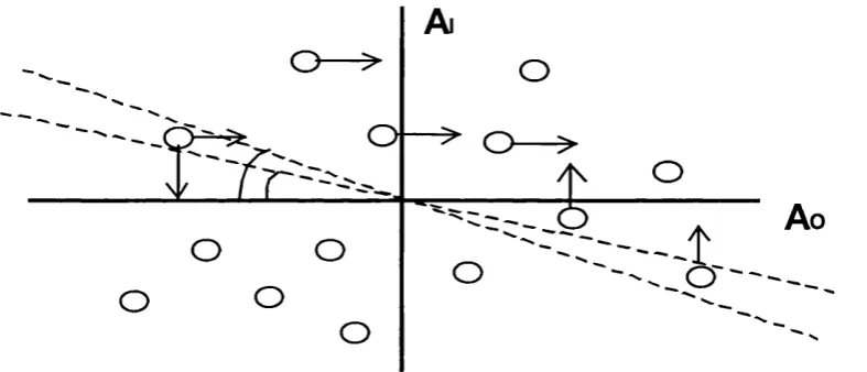
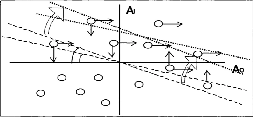
The key is therefore how Ph is constructed. The RA algorithm uses the following procedure, which requires a reverse connection matrix from the O to the H layer, to be discussed later.

1) Impose the input ?i and output ?o pattems simultaneously on the I and O layers respectively;

2) Compute the combined activation pattem on H layer

Ah'*^=Wih Pi + vj/WoH Po (Eq. 4.1)

where Wih and Won denote the weight matrices from I=>H, H=>0, and 0=>H; and Y is a pre-set, non-negative number called the reverse activation strength.

3) Produce binary activity pattem Ph* by way of the following:

Ph* 0)^1 only if Ah^ (j) is one of the top W activation amongst all j= l,2 ,.. .Nh,

where W is a pre-set number, fixing the activity ratio of the intemal representation.

4.1.2 The Key Elements and the Biological Plausibility o f RA

The Reverse Activation Matrix

The Two fundamental questions arise about the reverse activation matrix Wqh- What determines the individual weights, i.e. the form of the matrix Wqh? And how is its

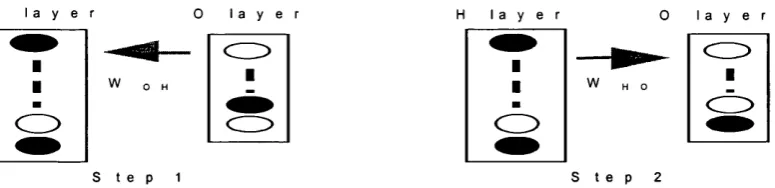
The basic requirement for the W q h is that it should be an adequate inverse to the

forward matrix. That is, on the 2-layer network of the H and the O layer, given any output pattem, the reverse matrix should be capable o f producing a pattem on H which produces the output itself via the forward matrix. This is because the purpose o f the reverse connections, when activated by a desired output pattem, is to shift the activity on the H layer towards a pattem that will reproduce the output pattem via the forward matrix. The best choice o f W q h in fact appears to be the transpose of W h o, as

discussed in Chapter 4.

Once teaming of a set of I-O mappings has taken place, only the forward connections are taken into account in assessing teamed performance. The reverse connections may be able in principle to contribute to improving the quality of an output pattem through dynamic interplay of the H and O layers during recall, but this would take time to settle and only the correctness of a teamed output on the first step of such a dynamic process is actually considered here.

Reverse Activation Strength

The reverse activation strength v|/ is an important tuneable parameter for the RA

algorithm. It is needed partly to counteract arbitrary scaling o f the I=>H weights

H=>0 connections: when vi/=0, the input representation remains unchanged and

learning is entirely carried out on Who; whereas with vj/=oo, much o f the learning involves changes in Wih, which may result in a new representation that requires little if any change to W h o to produce the desired output.

In the initial simulations of RA, \\f is fixed prior to training and remains fixed throughout the epochs. It is necessary to try out different values to determine the optimal range (rather like tuning for optimal step-size or momentum in BP). An alternative version selects \\j randomly from a pre-determined range prior to each superposition of inputs and outputs, so that v|/ changes every time it is used. The

advantage of the latter is that it obviates the need to tune \\j. It is interesting that this seems to work almost as well as employing a constant and optimal \\j.

How could Y be modulated in a biological context? Two possibilities are through effects o f diffuse neuromodulators and, perhaps more simply, by varying the strength with which the desired output pattern is activated. The latter mechanism strictly contravenes the simplifying assumption made in the model that neurons are binary, but it is of course quite feasible with more realistic neurons that have variable firing rates

Binarisation and Activity Ratio

The binarisation procedure is quite crucial in the construction of the internal representation. It is done by fixing the activity ratio o f the H layer. Then any activation pattern is binarised by allowing only the few most-activated cells to be ‘on’. Why is this necessary?

procedure must be to include the ‘good’ cells (whatever that means) and exclude the ‘bad’ ones. RA amounts to saying that the way to measure ‘goodness’ is via the ‘combined activation’ defined in the (Eq. 4.1). As such the absolute value of the activation o f each cell has little relevance in determining if a cell should be included in a representation or not because the activation is subject to arbitrary scaling. It is the relative order of activation that matters to the RA construction procedure.

As a result, fixing the activity ratio of the H and O layer is inevitable so that only the top few cells are allowed to be ‘on’. This is referred to as ramped binarisation. This makes the activity ratio on the H layer a tuneable parameter, providing a perfect opportunity to study the effect (on performance) of different activity ratio constraints for internal representations. As such, the RA procedure is a way of solving a given mapping task by constructing internal representations of a given activity ratio.

This binarisation procedure is also applied during recall on both the H layer and the O layer, for consistency. The behaviour of the network is more robust as a result.

A Non-gradient Descent Method

One key difference between RA and BP or other gradient descent methods is that the internal representations constructed are not driven by output-errors. The input and output mappings alone determine directly what the appropriate internal representations should be. Not having a defined error-surface in which to descent, it is hard to study the method analytically. For instance, it is not clear why the process should converge let alone learn anything at all.

Generalisation to Multiple Layers

of the dynamics resulting from the bi-directional linkage between the layers, keeping the input and output layers clamped. In Section 4.4, it is proved that such fixed points always exist and explained how this is consistent with the RA for 3-layer networks.

Biological Plausibility of Assumptions

The process of improving representations on the H layer is essentially a matter of recruiting 'better' cells for the purpose of generating the desired output and dropping 'bad' cells. One could look on this as analogous to learning to notice features of an input that lead you to the right conclusions about it, and learning to ignore features that lead to the wrong conclusions, based on previous learning. The criterion for 'good' cells is that they are strongly activated from (and by inference associated with) the correct output as well as the input, using a suitable reverse weight matrix. In fact the reverse matrix adopted for the simulations (the transpose o f the forward weights) is likely to be one o f the more simple to establish biologically, since the reverse connection between cells Oj and Hk is the same as the forward connection between the same cells, and this might be expected on the basis of simple associative (Hebbian) synaptic modification. Reciprocal connections from higher level centres are very common in the brain (e.g. Mumford, 1991,1992; Lee et. al. 1998), though their properties in relation to forward connections are not generally known.