The analysis of multivariate failure time data with application to multiple endpoints in trials in HIV infection

The Analysis o f M ultivariate

Failure Tim e D ata w ith

A pplication to M ultiple Endpoints

in Trials in H IV Infection

This work is presented as a thesis for the degree of

D O C T O R OF P H IL O S O P H Y

in

M edical S ta tistics

at the

Faculty o f C linical Sciences

U n iv ersity C ollege L ondon

by

A n n Sarah W alker

MRC HIV Clinical Trials Centre University College London Medical School

The Mortimer Market Centre

ProQuest Number: 10016142

All rights reserved

INFORMATION TO ALL USERS

The quality of this reproduction is dependent upon the quality of the copy submitted. In the unlikely event that the author did not send a complete manuscript and there are missing pages, these will be noted. Also, if material had to be removed,

a note will indicate the deletion.

uest.

ProQuest 10016142

Published by ProQuest LLC(2016). Copyright of the Dissertation is held by the Author. All rights reserved.

This work is protected against unauthorized copying under Title 17, United States Code. Microform Edition © ProQuest LLC.

ProQuest LLC

789 East Eisenhower Parkway P.O. Box 1346

‘Someday we’ll look back on all this

and plough into a parked car”

A C K N O W L E D G M E N T S

I would like to thank the following people:

Abdel Babiker

R uth Walker

Janet Darbyshire

A B S T R A C T

Endpoints currently in use in clinical trials in HIV infection are a composite which in­

clude death, clinical events, measures of quality of life, events based on laboratory markers

and adverse events. A composite endpoint, defined as the first occurrence of any one of a

set of events (including death), is generally accepted as appropriate for use in Phase III tri­

als of efficacy and safety, and is analysed using univariate failure time methods. However,

events in such a composite endpoint are often heterogeneous in their effect on subsequent

mortality, and also in their pathology, physiological system affected, and potentially their

response to antiretroviral treatm ent. Statistical methods for the analysis of such multi­

variate failure time d ata fall into three broad classes - marginal, frailty and conditional

models. A new semi-parametric marginal model based on Poisson regression for failure

d ata and GEE is developed, and the use of correlation structures other than independence

investigated. This estimation process is compared in a simulation study with the standard

m ethod for multivariate failure time data based on a Cox partial likelihood. A new simple

binary frailty model is also developed using both param etric and semi-parametric baseline

hazards. Various estimators of the semi-parametric and param etric hazard are compared

in a simulation study. Finally, these methods are applied to data from the D elta and Con­

corde trials. Initially, AIDS events are split into broad classes based on subsequent risk of

death, and then multivariate failure time methods applied to these classes. Combination

antiretroviral therapy can be shown to delay progression to more severe AIDS events com­

pared to monotherapy. These late events are generally untreatable and prophylaxis is not

available. The effect of treatm ent on individual AIDS events varies considerably. More than

one composite endpoint can also be analysed using these methods, providing an overall test

Table o f Contents

1

In tro d u ctio n

17

1.1 Composite e n d p o in ts ... 18

1.1.1 D e a th ... 18

1.1.2 Late clinical events ...18

1.1.3 Less serions clinical events ... 19

1.1.4 Laboratory m arkers... 20

1.2 Multiple events and multiple e n d p o in ts...20

1.3 Statistical m e th o d s... 22

1.4 N o ta tio n ... 22

1.5 Summary of new fin d in g s...23

2

A n alysis o f m ultivariate failure tim e d a ta

30

2.1.1 Extension of the univariate proportional hazards m o d e l... 31

2.1.2 Extension of the univariate Poisson m odel... 32

2.1.3 Using marginal m odels...33

2.2 Frailty m odels... 34

2.3 Conditional and m ultistate models ... 35

2.3.1 Conditional model for recurrence data based on independent in c re m e n ts 35 2.3.2 Extension of the conditional model for recurrence d a t a ... 36

2.3.3 M ultistate models ... 40

2.3.4 Using conditional and m ultistate m o d e ls ... 42

2.4 O ther methods and models not considered in the th e s is ... 43

2.4.1 Multilevel m odels... 43

2.4.2 Accelerated failure time (AFT) m odels... 44

2.4.3 M ethods based on joint distributions... 45

2.5 Comparison of methods in the lite ra tu re ...46

2.6 M ethods of adjusting for multiple endpoints in th e lite ra tu re ... 48

2.6.1 Global t e s t s ...48

2.6.2 Test procedures... 50

3

M arginal m od els for m ultivariate failure tim e d a ta u sin g a

w orking assu m p tion o f in d ep en d en ce

53

3.1.1 P artial likelihood with a working assumption of ind ependence... 53

3.1.2 Full likelihood with working assumption of independence and param etric baseline h a z a rd s ...58

3.1.3 Bootstrapping with a working assumption of independence...59

3.2 Semi-parametric marginal model for multivariate failure tim e d ata based on Poisson G E E ... 60

3.2.1 Poisson GEE with known baseline h a z a r d ...60

3.2.2 Poisson GEE with a param etric baseline h a z a r d ... 62

3.2.3 Poisson GEE with the Breslow estimate for the cumulative baseline hazard . . . 63

3.2.4 Variance estimators for ^ ... 72

3.2.5 Invariance under shift in location of covariate m e a n ... 72

3.2.6 Some issues involved in fitting Poisson G E E ... 74

3.3 Modelling event specific covariate effects with event specific baseline hazards . . . 76

3.3.1 Competing r is k s ...78

3.4 Simulation studies: design ... 79

3.4.2 Censoring pattern and the baseline h a z a r d ... 80

3.4.3 Covariate desig n...81

3.4.4 Model parameters ...82

3.4.5 Analysis methods co m p ared ...83

3.4.6 Implementation of analyses...83

3.5 Simulation St u d y( I ) : D ata simulated from a common regression coefficient with proportional m a rg in s ... 85

3.5.1 Weibull baseline h a z a r d ... 86

3.5.2 Breslow estimate for the baseline h a z a r d ... 87

3.5.3 Design effects... 98

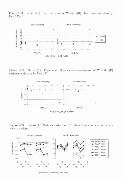
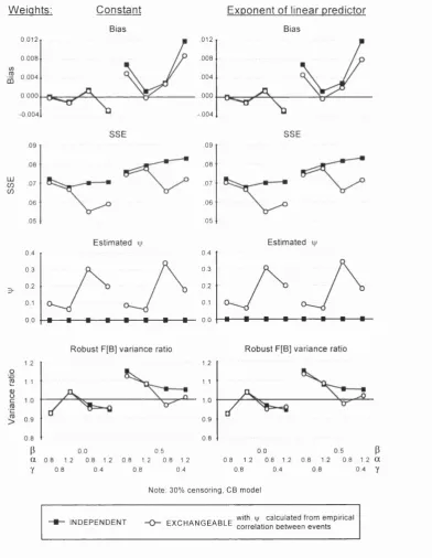
3.5.4 Comparison of WLW and F[B] robust variance estim ato rs... 98

3.5.5 St u d y( I): D ata simulated from a different baseline h a z a r d ...99

3.5.6 Comparison of two scenarios in St u d y(I) ... 101

3.5.7 Empirical relationship between estim ators... 101

3.5.8 Sensitivity analyses under S t u d y ( I ) ...102

3.5.9 Summary of St u d y(I) ...106

3.5.10 O ther parameters not varied in St u d y( I ) ... 108

3.6 St u d y(2): d ata simulated with category specific covariate effects and proportional m a rg in s ... 108

3.6.1 Sensitivity analyses under St u d y(2) ...110

3.7 St u d y(3): Alternative specification of DB d a t a ... 112

3.8 Performance under model m isspecihcation...113

3.8.1 Missing co v a ria te s... 114

3.9 S u m m a ry ... 116

M arginal m odels for m u ltivariate failure tim e d a ta u sin g

w orking correlation stru ctu res oth er th a n in d ep en d en ce

117

4.1.1 E fficiency... 118

4.1.2 Problems and underlying assumptions ... 119

4.1.3 Marginal models for multivariate failure time d ata with correlation structures other than in d e p e n d e n t... 120

4.2 Weighted Poisson GEE for multivariate failure time d a t a ...123

4.2.1 Comparison with weighted partial likelihood...124

4.2.2 Explicit form of the weighted GEE ...126

4.2.3 A simple example of bias from GEE with non-independent correlation s tru c tu re ... 127

4.2.4 Correction for b ia s ... 128

4.2.5 Estim ation of variances and GEE correlation p aram eters... 131

4.3 Simulations based on simple and expected w eights...132

4.3.1 Simple weights for St u d y( I): unit independent standard normal covariate design ...133

4.3.2 Expected weights for St u d y( I) : standard normal covariate designs... 135

4.3.3 Expected weights for St u d y(3): true correlation structure not exchangeable... 137

4.4 Invariance to a change in location of covariate m e a n ...138

4.4.1 0/1 cluster constant and unit independent covariate d esig n s...140

4.5 Comparison of GEE with independent and non-independent working correlation s tru c tu re s ...142

4.6 S u m m a ry ... 143

5.1 Review of frailty models for multivariate failure tim e d ata in the lite ra tu re . . . . 145

5.1.1 Frailty models with param etric baseline h a z a rd s ... 148

5.1.2 Frailty models with non param etric baseline h a z a rd s ...149

5.1.3 Frailty models with semi-parametric baseline h a z a r d s ...150

5.1.4 Laplace transforms ...152

5.1.5 Later developm ents...153

5.2 A binary frailty model for multivariate failure tim e d ata using the Poisson model ...154

5.2.1 Variance E s tim a tio n ...156

5.2.2 Param etric baseline h a z a rd s ...157

5.2.3 Semi-parametric estimation of the cumulative baseline h a z a r d ... 158

5.2.4 Revised variance calculation for semi-parametric profile cumulative h a z a r d ... 161

5.2.5 Testing for fra ilty ...161

5.2.6 Marginal hazard r a tio s ... 164

5.2.7 Identifiability... 165

5.3 Extensions of the Poisson binary frailty model ...168

5.3.1 Time dependent covariates with semi-parametric baseline hazard estim ation... 169

5.3.2 Covariate effects in the frail proportion of the population ... 170

5.3.3 Correlated rather than common binary frailtie s... 171

5.3.4 Multiple levels of clustering ...173

5.4 Binary frailty with the Cox proportional hazards m odel... 173

5.4.1 Comparison with counting process frailty m o d e ls ... 175

5.4.2 Relationship between Poisson and Cox binary frailty m odels... 175

5.4.3 Practical problems with the Cox binary frailty m o d e l...176

5.5 Simulations based on the Poisson binary frailty m o d e l... 178

5.5.1 The EM algorithm: speeding convergence... 178

5.5.2 Param eter sp a c e ...180

5.5.3 Convergence...181

5.5.4 Simulated d a t a ...182

5.5.5 Exponential baseline h a z a rd ...184

5.5.6 O ther param etric baseline h a z a rd s ... 185

5.5.7 Semi-parametric baseline h a z a rd s... 185

5.5.8 Performance of semi-parametric binary frailty model under frailty misspecihcation...188

5.6 Simulations based on the Cox binary frailty model ... 190

5.6.1 Comparison of Cox and Poisson binary frailty models for small d a ta se ts 191 5.7 S u m m a ry ...191

6

A p p lica tio n s to trials in H IV in fection

193

6.2 Issues in the analysis of multiple events in clinical tria ls ...196

6.2.1 Overall estimates for treatm ent effects across failure c a te g o rie s ...196

6.2.2 D eath censoring AIDS events... 197

6.2.3 Ties ... 199

6.2.4 Time-varying covariates...199

6.3 The Delta t r i a l ... 199

6.3.1 Design of the Delta trial ...199

6.3.2 Ranking of AIDS events based on subsequent m o rta lity ... 201

6.3.3 Differences between accepted and reported events in subsequent m ortality . . . 207

6.3.4 Interactions with treatm ent g r o u p ...208

6.3.6 AIDS events as separate failure categories...221

6.3.7 Including death in each failure categ o ry ... 236

6.3.8 Excluding death as a failure c a te g o ry ... 237

6.3.9 AIDS events as multiple failures of the same k in d ... 238

6.3.10 Combining more than one trial e n d p o in t...240

6.4 The Concorde t r i a l ... 242

6.4.1 Design of the Concorde tr ia l... 242

6.4.2 Ranking of AIDS events based on subsequent m o rta lity ...243

6.4.3 Effect of immediate treatm ent with AZT on different AIDS e v e n ts...245

6.5 S u m m a ry ... 249

D iscu ssion

252

R E F E R E N C E S

257

Appendix A

Marginal models with working assumption of independence

266

Appendix B

B1

B2

B3

B4

B5

Binary frailty models

269

Theoretical derivation of the binary frailty model in the

standard EM framework 270

Estimation of parameters of piecewise exponential baseline

hazard for the binary frailty model 273

Estim ation of parameters of Weibull baseline hazard for the

binary frailty model 274

Multiple levels of clustering 276

Variance estimation for binary frailty Cox model 278

A p p e n d ix C SAS p rog ram s 279

C l Semi-parametric GEE with working assumption of independence 280 C2 Semi-parametric GEE with non-independent working

assumption and expected weights 285

C3 Semi-parametric binary frailty model with profile estim ate of

the cumulative baseline hazard 294

Appendix D

Marginal simulation results using a working assumption of

independence

D1 St u d y( I ) : CB data, CB model with Weibull basehne hazard 308

D2 St u d y( I ) : CB data, CB model with Breslow hazard 310

D3 St u d y( I ) : CB data, CB model with Breslow hazard —

estimation of 318

D 4 St u d y(I): CB data, CB model with large non-centered cluster

constant covariate 319

D5 St u d y(I): DB data, DB model with Breslow hazard 320 D 6 St u d y(I): CB data, CB model with Breslow hazard — large \f3\ 326 D7 St u d y(2); DB data, DB model with Breslow hazard 329 D 8 St u d y(3): DB data, misspecihed DB model w ith Breslow

hazard 333

D9 St u d y(4): DB data, misspecihed DB model with Breslow

Appendix E

Marginal simulation results using non-independent

working correlation structures

335

E l St u d y(I): CB data, CB model with Breslow baseline hazard — simple weights and various estimators of ijj w ith unit

independent covariate design 336

E2 St u d y(I): CB data, CB model with Breslow baseline hazard

-expected weights and various estimators of ^ 337 E3 St u d y(3): DB model with Breslow baseline hazard - expected

weights and estimated by corr {Aij, A^k) 338

E4 St u d y(I): CB data, CB model with Breslow baseline hazard - expected weights and ijj estimated by corr ( A ij,A ik ) from a

model invariant to change in location of covariate mean 340

Appendix F

Frailty simulation results

344

F I Exponential baseline hazard 345

F2 Weibull and piecewise exponential baseline hazards 346

F3 Breslow baseline hazard 348

F4 Misspecified frailty distribution with profile (Breslow) baseline

List o f Tables

3.1 St u d y( I ) : Bias and sampling standard error (SSE) of ^ (o; =

1.2, CB model) 89

3.2 St u d y( I ) : Bias and sampling standard error (SSE) of ( a = 1.2,

CB model) 89

3.3 St u d y( I ) : Variance ratios of the mean WLW and F[B] variance

estimates to the sampling variance of P (60% censoring, a = 1.2, CB model) 91

3.4 St u d y(I): Size/power of the logrank test based on WLW and F[B] variance

estimates (60% censoring, a = 1.2, CB model) 91

4.5 Gain in efficiency for standard normal covariate designs from simple and

expected weights with exchangeable GEE correlation structure 135 5.6 Comparison of Cox and Poisson binary frailty models for small datasets 192 6.7 Hazard ratios for subsequent mortality associated with accepted AIDS

events in the Delta trial 205

6.8 Hazard ratios for subsequent m ortality associated with reported AIDS

events in the Delta trial 206

6.9 Interactions between treatm ent group and occurrence of AIDS events for

subsequent m ortality in the Delta trial 209

6.10 Comparison of log HR and their standard errors for progression to AIDS or

death from independent and non-independent GEE 219

6.11 Log HR for the overall treatm ent effect and their standard errors in

participants entering D elta without AIDS 221

6.12 Hypothesis tests for treatm ent effects 226

6.13 Overall estimates of treatm ent effect — all participants 227 6.14 Log HR for the overall treatm ent effect and their standard errors in the

D elta trial 236

6.15 Log HR for the overall treatm ent effect and their standard errors in the

List of Figures

1-1 Potential event histories experienced in an HIV clinical trial 21 3-1 St u d y(I): Variance ratios from unadjusted and adjusted estimates for the

variance of ^ from a Weibull model with cluster constant covariates 86

3-2 St u d y(I): Bias and sampling standard deviation for cluster constant

covariate designs using Weibull and Breslow baseline hazards 88 3-3 St u d y(I): Variance ratios from cluster constant covariate designs 90 3-4 St u d y(I): D istribution of variance estimates for cluster constant standard

normal covariate design 93

3-5 St u d y( I ) : Distribution of variance estimates for the cluster constant 0/1

covariate design 93

3-6 St u d y(I): Variance ratios from uniform cluster constant covariate design

with covariate centered at zero prior to analysis 94 3-7 St u d y(I): Variance ratios for unit-varying covariate designs 95 3-8 St u d y(I): Distribution of variance estimates for the unit-varying

case-control covariate design 97

3-9 St u d y(I): Distribution of variance estimates for unit independent standard

normal covariate design 97

3-10 Design effects from all covariate designs 99

3-11 St u d y( I ) : Distribution of WLW and F[B] robust variance ratios by

Va r^ Xi j 100

3-12 St u d y( I ) : Percentage difference between robust WLW and F[B] variance

estimates by V a r 100

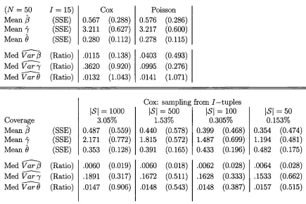
3-13 St u d y( I ) : Variance ratios from DB data from standard normal covariate

designs 100

3-14 St u d y(I): Difference between sampling, naive and robust variances for small (3 and small 7 with the unit independent standard normal covariate

design 103

3-15 St u d y(I ): Bias as % of MSE for \(3\ >0.5 104 3-16 St u d y(I ): Naive and robust variance ratios from the unit independent

standard normal design 105

3-17 St u d y(I): Robust variance ratios for \!3\ > 0.5 105 3-18 St u d y(I): Variance ratios for high correlation and large sample size with

\(3\ = 2 106

3-19 St u d y(2): Robust WLW and F[B] variance ratios for cluster constant

covariate designs 111

3-20 Variance ratios from cluster constant standard normal covariate design w ith

category specific covariate effects 111

3-21 Naive and robust variance ratios for St u d y( I ) cluster constant covariate

designs with category specific effects 111

3-22 Comparison of bias as %MSE from the three misspecified models with

standard normal covariate designs 115

4-1 St u d y(I): g e e with exchangeable working correlation and simple weights

— standard normal unit independent covariate design 134

4-2 St u d y( I ) : g e e with exchangeable working correlation and expected

weights — standard normal covariate designs 136

when margins are not proportional — standard normal covariate designs 138

4-4 St u d y(I): g e e with exchangeable working correlation and expected

weights — 0/1 covariate designs 141

5-1 Bias and % MSE from semi-parametric binary frailty model w ith profile

estim ate of the cumulative baseline hazard 186

5-2 Median variance ratios from semi-parametric binary frailty model with

profile estim ate of the cumulative baseline hazard 187 5-3 Bias in ^ from misspecified semi-parametric binary frailty models with

profile estimate for the cumulative baseline hazard 189 5-4 Median variance ratios from misspecified semi-parametric binary frailty

models with profile estimate of the cumulative baseline hazard 190 6-1 Hazard ratios for subsequent mortality associated with accepted AIDS

events — for participants entering the D elta trial w ithout AIDS 203 6-2 Progression to AIDS or death (for participants w ithout AIDS at entry)

-competing risks 211

6-3 Progression to AIDS or death (for participants w ithout AIDS at entry)

-marginal model 212

6-4 Progression to AIDS or death (for participants w ithout AIDS at entry)

-binary frailty model 214

6-5 Unconditional hazard ratios from binary frailty model 217 6-6 Progression to AIDS or death (for participants w ithout AIDS at entry)

-m ultistate -model 218

6-7 Development of new AIDS events and death for all participants in the Delta

trial 223

6-8 D istribution of the estimated frailty from the binary frailty model with

separate treatm ent effects for each AIDS event and death 225 6-9 Correlation between log HR for each treatm ent comparison on each failure

category 225

6-10 Selection of unconditional hazard ratios from the binary frailty model with

failure category specific treatm ent effects (AZT experienced) 227 6-11 Development of a new AIDS event or death for all participants in the D elta

trial - combining treatm ent effects by severity of AIDS events 229 6-12 Unconditional hazard ratios from the binary frailty model w ith common

treatm ent effects by severity of AIDS events (AZT experienced) 229 6-13 Sensitivity of estimated treatm ent effects to the degree of correlation

between frailties within individual 231

6-14 Hazard ratios from interaction model with prior AZT exposure — combining

treatm ent effects by severity of AIDS events 231

6-15 Conditional hazard ratios from binary frailty interaction model with

treatm ent — combining treatm ent effects by severity of AIDS events 234 6-16 Development of a new AIDS events or death for all participants in the D elta

trial - combining treatm ent effects by clinical class of AIDS events 234 6-17 Hazard ratios for AZT-|-ddI vs AZT from models excluding and including

death before each AIDS event in each failure category 237 6-18 Hazard ratios for AZT4-ddI vs AZT using a “recurrence” model with

Definition HI for the failure categories 239

6-19 Hazard ratios for AZT4-ddC vs AZT using a “recurrence” model with

Definition HI for the failure categories 239

6-20 Hazard ratios for subsequent mortality associated with AIDS events in the

6-21 Hazard ratios for immediate versus deferred AZT on progression to AIDS

events and death in the Concorde trial 246

6-22 Progression to AIDS events and death in the Concorde trial — common

G L O S S A R Y

Abbreviations

AG - Andersen Cill (model)

ALR - alternative likelihood ratio (test)

ARC - AIDS related complex

AZT - zidovudine

BF - binary frailty (model)

CB - common baseline (hazard model)

CDC - Centers for Disease Control

CD4 - subset of T-lymphocytes (an immunological prognostic marker)

Cl - confidence interval

CP - Cai Prentice (model)

CPCRA - Community Programs for Clinical Research on AIDS

DB - different baseline (hazard model)

ddC - zalcitabine

ddl - didanosine

Def - deferred AZT

df - degrees of freedom

ECM - conditional expectation maximisation

EM - expectation maximisation

F[B] full derivative based on the Breslow estim ate for the cumulative baseline hazard

CEE - generalised estimating equations

CLM - generalised linear model

CLMM - generalised linear mixed model

HR - hazard ratio

lE E - independence estim ating equations

Imm - immediate AZT

IQR - interquartile range

LR - likelihood ratio

LSC - Liang, Self and Chang (model)

LWA - Lee, Wei and Amato (model)

MCMC - Markov chain Monte Carlo

ML - maximum likelihood

MSE - mean square error

NR - Newton Raphson

01 - opportunistic infection

P[B) full derivative based on the Breslow estim ate for the cumulative baseline hazard

PH - proportional hazards

PW P - Prentice, Williams and Peterson (model)

RMSE - root mean square error

SE - standard error

SSE - sampling standard error

In addition, the various AIDS-defining events will be abbreviated as follows —

PML - Progressive multifocal leucoencephalopathy NONHL - Non Hodgkin’s lymphoma

CERLYM - Prim ary cerebral lymphoma HIVENC - HIV encephalopathy

INDLES - Indeterm inate intracerebral lesions CERTOX - Cerebral toxoplasmosis

HIVWAST - HIV wasting

PGP - Pneumocystis carinii pneumonia KS - Kaposi’s sarcoma (all)

OESCAN - Oesophageal candidiasis EXPTB - Extrapulm onary tuberculosis

CROC - Cryptococcosis

CRSP - Cryptosporidiosis MISP - Microsporidiosis

MAI - Disseminated Mycobacterium avium intercellulare HSV - Herpes simplex virus disease

CMVRET - Cytomegalovirus retinitis

CMVOTH - Cytomegalovirus disease (not retinitis) CMV Cytomegalovirus disease (any site)

3t a n d D efinition of Sym bols

— — definition

àjk - Kronecker delta function

(S) - tensor product, such as :=

L - likelihood function

I - log likelihood function

U - score or estimating function

Failure time d ata

F - true failure time

C - censoring time

T - observed failure time, := min (F, C)

A - event indicator, := 1 if T = F and 0 otherwise

X - covariate vector

(t, A ,x ) - observed data

y ( t) - risk set indicator, := I ( T > t)

- risk set at time t, := {V(t) = 1} IV (t) - counting process, := I {T < t, A = 1)

M ( t) martingale associated with counting process N (t) : = N ( t ) - f * Y ( u ) A ( u ) d u

Æ W - predictable random covariate process

A(t) - hazard

K{t) - cumulative hazard function, := Jq A (n) du

Regression models for failure tim e data

S » (t)

S ' ( t )

S2(t)

a

-A

Marginal models

7

A B

i

w

Frailty models

U u

7

regression param eters := Ao(t) exp (mean)

weighted number at risk at time t, := Y Irçi)

weighted covariate mean at time t, := ^xp x) x

weighted covariate cross product at time t, := YliR{t) Gxp x) x x ^

Weibull shape param eter in baseline hazard Weibull scale param eter in baseline hazard

positive stable parameter, describing assocation of failure times within cluster

naive variance for the estimating function robust variance for the estimating function GEE working correlation m atrix

param eters of GEE working correlation m atrix

overall weighting m atrix in GEE with non-independent correlation structure

frailty covariate

param eter of continuous frailty distribution effect of binary frailty in the linear predictor probability of being frail in the binary frailty model

Throughout, multivariate failure time data is assumed to arise from i = \ .. .1 indepen­ dent individuals or clusters, with j = 1. ..Ui failure categories or units in each cluster

i. Glusters will be indexed by z,/,p; and units within clusters indexed by j , k , m , q .

Although d a ta from different clusters are assumed to be independent, within clusters both responses and covariates may be correlated. W ithout loss of generality we assume

7ii = J \/i. Covariates and responses for each item {ij) will be indexed by subscript ij.

Chapter 1

Introduction

A wide variety of endpoints are currently in use in clinical trials in HIV infection. A

participant is generally considered to reach a trial endpoint at the first occurrence of any

one of a set of previously defined events — such endpoints are therefore a composite. Events

after the first are ignored, at least in the main analyses of these trials. The events included in

a composite endpoint can show considerable heterogeneity, both in their effect on subsequent

m ortality and also in their effect on other measures such as quality of life.

This thesis investigates ways in which multiple events experienced by participants over

the course of a trial can be used more effectively, focusing primarily on th e joint analysis

of the multiple events contained in a composite endpoint. This involves the comparison

of m ultivariate failure time analysis methods (those described in the literature and some

extensions), and the application of these methods to treatm ent comparisons.

The methods axe applied to multivariate failure time d ata from two trials, Concorde

and Delta, covering a wide spectrum of HIV disease. Concorde was a trial of immediate

versus deferred therapy with zidovudine (AZT) in asymptomatic HIV infected individuals

(median CD4 at entry 455 cells per mm^) [26] . Delta was a trial of AZT monotherapy

versus combination therapy with AZT and either didanosine (ddl) or zalcitabine (ddC), in

participants either with symptoms of HIV disease or with CD4 below 350 cells per mm^

1.1

C o m p o site e n d p o in ts

Endpoints currently used in HIV clinical trials are often a composite of events which can

include death, serious clinical events (such as AIDS events), mild clinical events (such as

AIDS Related Complex (ARC)), measures of quality of life, adverse events and events based

on laboratory markers. Composite endpoints (defined as the first occurrence of one of a set

of clinical events including death) have generally been accepted as most appropriate in Phase

III type trials of efficacy and safety, and are analysed using univariate failure time methods.

Some problems, such as missing data, affect all types of event used in composite endpoints.

Some of the advantages and disadvantages specific to particular events are described below.

1.1.1

D e a th

U ltim ately the most im portant clinical endpoint is death. This endpoint avoids problems

of observer bias, all participants are at risk at all times, and no further events are possible.

The main disadvantage is th a t trials need to be large or of long duration in order to achieve

the necessary power, even in advanced HIV disease. Continued development of new and

potentially more active drugs makes the assessment of the relative effect of all combinations

on m ortality impractical. The likelihood of drug resistance in patients on the same regimen

for long periods also means th a t participants are likely to change therapy several times

before death. If there is a beneficial treatm ent effect on other clinical events occurring prior

to death then it may be unethical to continue a trial once this effect is known. In view

of these practical considerations, many trialists would find th e use of survival as the only

endpoint unacceptable except in very advanced HIV disease.

1.1.2

L ate clinical even ts

In view of the disadvantages of using death alone as the endpoint, a composite endpoint

clinical events should occur in the late stages of HIV disease, and should be associated

with severe immuno-suppression and be indicative of poor prognosis. AIDS is the most

commonly used criteria for late HIV disease, defined as the development of any one of a

set of opportunistic infections (OIs) and tum ours (for example, CDC defined criteria [16] ).

AIDS or death is a common trial endpoint. In participants entering a trial w ithout AIDS,

time to the first AIDS event is used. In participants with AIDS at entry the first new but

non-recurrent AIDS event is commonly used, due to difficulties in distinguishing between a

true recurrence of a previous AIDS event and a failure to treat a previous event successfully.

Although CDC criteria are used as a working definition of AIDS by clinicians worldwide,

they were designed for disease surveillance, and the various AIDS defining events differ in

their effect on subsequent m ortality and other measures such as quality of life [91] . In

addition, deciding whether a participant has reached an AIDS endpoint within a clinical

trial depends on a large set of criteria relating to the diagnosis (presumptive (based on

clinical findings) or definitive (based on pathological findings)). The extensive investigations

required are not always performed, or even appropriate in late disease. Only a subset of

all reported AIDS events are therefore classified as accepted (or definite/ probable) AIDS

events for the purposes of the trial (based on whether they fulfil the criteria for presumptive

or definitive diagnosis).

1.1.3

Less serious clinical even ts

Even including late clinical events in a composite endpoint with death, trials in early or

asym ptom atic HIV infection may need to be large or of long duration to achieve the neces­

sary power. Therefore, symptomatic HIV disease not fulfilling the definition of AIDS (such

as ARC) has also been used in composite endpoints in some trials. The m ajor disadvan­

tages of using less serious clinical events are th a t they may be highly subjective as it is

difficult to specify diagnostic criteria, and therefore tend to be prone to observer bias (for

poorly documented and hard to validate.

1.1.4

L ab oratory m arkers

In view of the problems associated with using less serious clinical events in endpoints, trials

have also been designed to include changes in laboratory markers (such as CD4 cell counts

or viral load) in either primary or secondary endpoints. Markers are not prone to subjective

or observer bias: however, the underlying assumption is th a t the marker is a surrogate for

the clinical disease process. Prentice [101] set out criteria th a t a laboratory marker should

satisfy for it to be a surrogate marker for a clinical endpoint; in essence, a test of the null

hypothesis of no treatm ent effect on the laboratory marker must be a valid test of the

null hypothesis of no treatm ent effect on the clinical endpoint. Although CD4 cell count

has been validated as a prognostic marker in many studies (for example [35] [98] ), it has

been shown to be an inadequate surrogate for death and progression to AIDS or death (for

example [26] [76] [120] ).

1.2

M u ltip le e v e n ts an d m u ltip le e n d p o in ts

P articipants reach a trial endpoint when they develop their first clinical event satisfying

the endpoint criteria. W hen the effect of treatm ent on the trial endpoint is assessed, no

distinction is made between the different clinical events included and no use is made of any

subsequent events experienced by each individual. Some problems inherent in this analysis

of composite endpoints are made clearer by considering the potential event histories for

participants in a trial shown in Figure 1-1 (reproduced from Neaton et al [91] ).

The composite endpoint analysis ranks participants in the order (1 — 2 — 3), although

the number of events experienced under follow up implies the reverse order, and the relative

severity of first events would suggest a ranking (2 — 3 — 1). Approaches which attem p t to

Figure 1-1

Potential event histories experienced in an HIV clinical trial

=5

2

0_

candidiasis

K---PML

- K I

PCP C M V -K— K---K— o

candidiasis

A ID S e v e n t

o end o f follow up

■ d e a th

Time from randomisation

subsequent) satisfying the trial endpoint criteria. Considering all events as failures of the

same kind leads to recurrence models. Alternatively, the severity of each event satisfying

the trial endpoint criteria can be taken into account, where severity is ranked either by the

effect on subsequent mortality, or using subjective opinion from patients or clinicians, or by

some other measure such as quality of life. Both these approaches are implemented through

m ultivariate d ata analysis.

In some trials, attem pts have already been made to address the problem of endpoints

which are a composite of multiple heterogeneous events w ithout resorting to complicated

m ultivariate methods of analysis. In the Alpha [2] and D elta trials, only a subset (although

the majority) of the CDC AIDS defining events were used to define the trial endpoint of

AIDS to exclude events with better prognosis. The Delta trial also used a trial endpoint

of “advanced” AIDS, based on unpublished work on the prognostic effect of various AIDS

events using d ata from the Alpha trial [52] . However, even with careful definition of

endpoints new subsequent events meeting the endpoint criteria have generally been excluded

from analyses, even though they are possibly more severe and may be associated with a

higher risk of death.

M ultiplicity also arises as most trials use more than one endpoint to assess treatm ent

efficacy (for example, both death and AIDS or death). Each endpoint is analysed and

generally be related. There is rarely any indication of how potentially varying estimates

of treatm ent effect should be combined, or whether the effect of treatm ent really differs

significantly across the endpoints or not. This is essentially an issue of multiple testing

[100] , and relies on the estimation of the correlation between treatm ent effects on different

endpoints provided by multivariate failure time d ata analysis.

1.3

S ta tistic a l m e th o d s

S tandard methods for the analysis of failure tim e d a ta [30] assume th a t each individual

experiences at most one failure and th a t the failure times of different individuals are indepen­

dent. When multiple events for each individual are analysed, a naive analysis assumes th a t

all the different failure times of the individuals in the population are statistically indepen­

dent (given the covariate values). The precision of estimates obtained using this assumption

will generally be overstated because the failure times from the same patient are correlated,

and the methods will assume th a t there is more information than there really is. However,

the interdependence of event times may not ju st be a nuisance param eter which has to be

taken into account in the estimation of the covariate (treatm ent) effect — the degree of

dependence may itself be of intrinsic interest. Models for multivariate failure time d a ta fall

into the classes of marginal, frailty and conditional models. In the context of clinical tri­

als, marginal and frailty models are most appropriate in th a t the random isation balance is

preserved. Emphasis will therefore be placed on these methods. Semi-parametric marginal

and frailty models are developed, and compared w ith existing methods by simulation and

application to trial data.

1 .4

N o ta tio n

Throughout, multivariate failure time d ata is assumed to arise from i = 1 . . . / indepen­

Although d ata from different clusters are assumed to be independent, within clusters both

responses and covariates may be correlated. W ithout loss of generality we assume rii = J Mi.

Covariates and responses for each item {ij) will be indexed by subscript ij. Clusters will

be indexed by 2, and units within clusters indexed by j , k , m , q . Explicit ranges for

sums are not given in general. Likelihood functions will be denoted L, and log likelihood

functions by I. Definitions will be indicated by :=. Vectors will only be indicated using an

underbar where this is required for clarity. 6jk is the Kronecker delta function. Superscript

® denotes tensor product, such as = xx'^ .

For failure time models the hazard function will be denoted A(t), with cumulative hazard

A{t) = f ^ X ( u ) d u . The observed d ata are (t, A, x) , where t is the failure time, A the

censoring indicator and x the covariate vector. If A = 0 then the event did not occur and

t is a censoring time; otherwise if A = 1 then the event occurred and t is a true failure

time. Risk set indicators are denoted Y {t) = I { T > t), and R{t) = {Y {t) = 1} denotes

the risk set at tim e t. The corresponding counting process is N {t) := I {T < t, A = 1) and

the predictable random covariate process is X (t) (fixed at t given the history up to but not

including t ) .

1.5

S u m m a r y o f n ew fin d in gs

Inference from marginal models for multivariate failure time d ata can be made from gen­

eralized estim ating equations (GEE [74] ) using the Poisson formulation for failure time

data. The dependent variable is the censoring indicator and the regression is conditional

on an offset which is the log of the cumulative baseline hazard. Previously such G EE had

been based on param etric forms for the baseline hazard (such as exponential or Weibull):

in the thesis, semi-parametric inference based on the Breslow estimate of the cumulative

baseline hazard is developed both for independent and non-independent working correlation

Under a working assumption of independence, the param eter estimates from the semi-

param etric GEE are shown to be identical to those obtained from the standard multivariate

partial likelihood estimates of Wei, Lin and Weissfeld (WLW [124] ). However, two different

variance estim ators can be constructed based on the GEE, both with naive and robust

forms. The first is the standard GEE variance estim ator based on the Poisson likelihood

and thus considers the cumulative baseline hazard fixed with respect to the regression

param eters (P[Bj). This estim ator is therefore likely to underestim ate the variance because

the semi-parametric hazard depends on the regression param eters. In addition, this variance

estim ator is shown not to be invariant to a change in location of the covariate mean. A

second variance estim ator can be constructed which includes variation from the cumulative

baseline hazard in the estimation of the variance of the regression coefficients (F[B|). This

variance estim ator is invariant to a change in location of the covariate mean. However,

it does not derive directly from the Poisson GEE — it is the variance estim ator from

related estim ating equations which are not solved conditional on the offset (cumulative

hazard) being independent of the regression param eters. The difference between these F[B]

estim ating equations and the standard GEE (or partial likelihood) is shown to be O {(3) for

regression param eters /?.

The WLW variance estimators are equivalent to the P[B] variance estimators with the

covariates replaced by covariates centred around their weighted mean in th e current risk set

(weights equal to the exponent of the linear predictor). In contrast F[B] variance estimators

centre the covariates around a smooth of these weighted means over all risk sets up to and

including the current risk set, with most weight given to the most recent risk sets. Therefore

when Z$> 0, the expected covariate values differ across risk sets, and the F[B] variance

estim ator would be expected to differ substantially from the WLW variance estimator.

Simulation studies based on multivariate failure d a ta from a positive stable frailty dis­

tribution are used to investigate the performance of the variance estimators. The semi-

on the true param etric baseline hazard (Weibull) in the GEE. No significant bias in the re­

gression param eters was found in any simulation study. The relative performance of the

naive and robust variance estimators of all three types depends mainly on th e covariate de­

sign, although the magnitude of the difference also depends on the association between the

failure categories. The robust variance estimators are significantly closer to the sampling

variation th an the naive estimates except when the covariates are independent within d ata

clusters: however, the variation in the robust variance estimators was considerably larger

th an th a t in the naive variance estimators. As a consequence the root mean square error of

th e robust variance estimators is almost twice th a t of the naive variance estim ators when

covariates are independent within clusters. Sensitivity analyses show th a t the difference

between WLW and F[B] variance estimators clearly increases with increasing variance of

th e linear predictor: whereas WLW consistently underestim ates the sampling variance by

around 10% (a similar figure to th a t described elsewhere in the literature), F[B] overesti­

m ates the sampling variance as the variance of the linear predictor increases, approximately

independently of the correlation between failure categories, but with overestimation increas­

ing as censoring decreases. In addition, the simulation studies show th a t the naive variance

estim ators do underestim ate the sampling variance when covariates are independent within

cluster and the covariate effects are large. Both WLW and F[B] variance estimators per­

form similarly under model misspecification, both estim ating the sampling variation in /?

reasonably closely.

In the context of clinical trials, participants experience various events and interest lies in

estim ating the effect of treatm ent on the development of events in different failure categories.

T he marginal models are therefore specified by failure category specific baseline hazards

and covariate effects. W ith these models, the regression param eters and their standard

errors are shown to be virtually identical to those from univariate models provided th a t the

proportional hazards assumptions hold at least approximately in the margins. The increased

between the failure category specific treatm ent effects, which are effectively estim ated at

zero in the univariate models. This is dem onstrated in simulation studies. In clinical trials

it is likely th a t the treatm ent effect will be moderate, and the treatm ent group indicator

clearly has a low variance so th a t F[B] variance estimators should be reasonably accurate

and less conservative than the WLW estimates.

In theory Poisson GEE with the Breslow estim ate of the cumulative hazard is easily

extended to working correlation structures other than independence, with the aim of find­

ing more efficient estimates of the regression parameters. Cai and Prentice had extended

the independence working model based on partial likelihood to more general correlation

structures using the counting process formulation [13] . The weighting m atrix suggested

is th e inverse correlation of the martingale processes. Poisson GEE with non-independent

working correlation is shown to lead to similar estimating equations but with a different

and non-symmetric weight matrix. Furthermore, the partial likelihood variance estimators

depend on the derivative of the weight m atrix with respect to the regression parameters,

whereas the GEE variance estimators (P[Bj and F[Bj) take comparatively simpler forms.

However, it is easily shown th a t the Poisson GEE with non-independent working correla­

tion are biased, because the weights and the residuals are correlated through the observed

failure time. This is a consequence of the nature of multivariate failure time data, where

the responses (censoring indicators) are non-trivially related to the observed failure times

(the minimum of censoring and true failure times). The bias in the GEE is removed by

replacing the weight m atrix which is a function of the cumulative baseline hazard with a

fixed m atrix, or by a m atrix which only depends on the linear predictor (not the cumulative

hazard), or by taking the expectation of the cumulative hazard function. W hen covariates

are constant within cluster (such treatm ent group indicator as in the context of a clinical

trial), the first two weighting methods lead to identical estimating equations to the inde­

pendence working assumption. Taking expected weights requires param etric specification

m artingale correlation proposed by Cai and Prentice. Possible distributions which can be as­

sumed for the pairwise survivor functions include gamma and positive stable frailty models.

However, standard statistical software for GEE cannot be used with any of these weighting

methods. Simulation studies based on the same positive stable frailty distribution show

th a t when covariates are independent within cluster the three different weighting methods

lead to gains in efficiency of up to 45% compared with the independence working model,

with largest gain when the association between failure categories is highest, as expected. In

comparison, using the expected weights with a cluster constant covariate there was virtually

no difference in. sampling variation of j3 compared with the independence working model.

The G EE with non-independent working correlation are shown to be invariant to a change

in location of the covariate mean only in expectation, similarly to the weighted partial

likelihood of Cai and Prentice. This is a consequence of the lack of intercept in the GEE

which would be sufficient to ensure invariance to a change of covariate mean (thus, using

a parametric baseline hazard the GEE are invariant as the intercept is the log of the scale

param eter in the baseline hazard). Consideration of GEE with non-independent correlation

structure and an intercept leads to an estimating equation for (3 which is invariant to change

in location of the covariate mean, and is equivalent to estimation with all covariates centered

around their weighted mean prior to analysis.

Frailty models provide an alternative method for adjusting for association between fail­

ure categories within cluster. Various frailty models have been proposed for both semi-

param etric and param etric baseline hazard estimation in the literature (for example [66]

[48] ): however, semi-parametric estimators to date are not easily implemented in standard

statistical software. A new semi-parametric binary frailty model is developed in the thesis,

in which the unobserved covariate conunon to all units within each cluster is assumed to be a

binary covariate. This is an extension of the simple binary frailty model for binary responses

[7] to semi-parametric models for failure time data. The frailty is assumed to act additively

frail is 6, both to be estimated. Estimation proceeds via Poisson regression based on the

EM algorithm, with variance estimates constructed from the unconditional log likelihood.

Profile estim ation of the cumulative baseline hazard is shown to be the only m ethod of

semi-parametric inference which produces unbiased estimates and also preserves the correct

correspondence between (7 ,0) and (—7 ,1 — 0) space. A revised variance estim ate includes

variation from the profile estimate of the cumulative baseline hazard, based on contribu­

tions to the hazard at every distinct event time. Unconditional hazard ratios (averaged over

frailty) are constructed for comparison with the hazard ratios from the marginal models.

However, these unconditional hazard ratios are now a function of time. The binary frailty

model is easily extended to discrete rather than binary frailties, to correlated rather than

common frailties, and to multiple levels of clustering. In contrast, use of a binary frailty in

the partial likelihood proportional hazards regression model is shown to be impractical, as

the estim ating equations depend on summation over all possible distributions of the binary

frailty in the clusters in the population.

Simulation studies show th a t EM convergence can be considerably speeded by using

multicycle EM gradient algorithm followed by direct Newton-Raphson maximisation with

step-halving. Bias in all parameters (regression and frailty) is relatively small using the

profile estim ate for the cumulative baiseline hazard, although there is considerable variance

underestim ation for the frailty parameters. The adjusted variance estim ate improves the

variance estimation. The binary frailty model performs reasonably well under misspecifica­

tion of the frailty distribution (gamma or positive stable) provided th a t either (3 = 0 01 the

variance of the frailty distribution is not large.

Both marginal and frailty models are then applied to d ata from the Concorde [26] and

D elta [32] trials, using a variety of models to try and explore the patterns in treatm ent

effects across different AIDS-defining events. In both trials, the only significant variation

in treatm ent effect consistently found in both marginal and frailty models appears to be

with monotherapy appears to increase as the AIDS events become more severe, whereas in

Concorde the treatm ent effect of immediate AZT compared with deferred AZT appears to

decrease w ith severity of AIDS event. However, there is a significant interaction between

the effect of the binary frailty and treatm ent group in some models, leading to a different

pattern of effects from the marginal models when this interaction is ignored. In addition,

hazard ratios from the binary frailty model appear to be harder to interpret as they vary over

time (the conditional hazard ratios cannot be interpreted across participant). Comparison

of hazard ratios for the overall effect of treatm ent over the different AIDS events from

the marginal models using various methods of calculation (linear combination by minimum

variance or severity weighting, or common model) dem onstrate th a t in these trials there is

little reduction in standard error from including extra events compared with hazard ratios

from a first event analysis. This is likely to be a consequence of the specific p attern of

treatm ent effects, w ith the greatest effect of treatm ent on the least commonly occurring

Chapter 2

A nalysis o f multivariate failure tim e data

In m ultivariate failure time data, times to different (and correlated) events are grouped into

independent clusters. W ithin clusters, the different categories of event (units) take one of

two forms. Failure/event category will be used generically to describe either

♦ m u ltip le fa ilu re s o f d iffe re n t k in d s: for example, a set of AIDS defining events.

Individual patients correspond to clusters, the AIDS events correspond to units within

clusters and each cluster therefore contains the same number of units because each patient

is at risk for each AIDS event. The failure processes act concurrently, and at any time

any cluster (individual) can experience failure in any unit (AIDS event).

♦ m u ltip le fa ilu re s o f t h e sa m e k in d : for example, recurrences of the same failure, or

in a more general setting than HIV clinical trials, the occurrence of a disease in families.

For recurrences, individual patients correspond to clusters and different recurrences cor­

respond to units within clusters. In theory, a cluster (individual) should only be at risk

in the j t h unit (recurrence) after the {j — 1) th unit has already failed. More generally,

for familial diseases, families correspond to clusters, and family members correspond to

units w ithin the clusters. Any cluster (family) can experience failure in any unit (family

member) at any tim e and units are essentially exchangeable. In either case, different

clusters may have different numbers of units.

A triple {tij, Aij^x^j) is observed for each unit in each cluster. D ata from different

clusters, (1%, A%), are assumed to be independent and identically distributed, where

from the analyses, these covariate d ata are assumed to be missing completely at random

[107] . All m ethods of analysis also assume independent and non-informative censoring [4] .

Heuristically, conditionally on covariates, the instantaneous failure probabilities should be

identical w ith and w ithout observations on the censoring time, and the likelihood for items

censored in [t,t -\- dt) should not be a function of the regression param eters given the risk

set at t and the items failing at t.

M ethods of analysis of multivariate failure time d ata include marginal, frailty and con­

ditional models. Marginal methods of analysis specify models for the effect of covariates

on the hazards for each of the individual failure categories (the margins), adjusting the

estimates for the fact th a t each participant is observed for more than one event and all the

event times are correlated without specifying models for this correlation. The association

between the events is regarded as a nuisance param eter. Frailty models account for the

dependence between the events by the introduction of unobservable random effects into the

marginal hazards. Conditional methods explicitly model the association between various

events and are thus associated with loss of randomisation balance. Wei and Glidden [123]

provide an overview of methods available for the analysis of m ultivariate failure time data.

2 .1

M a rg in a l m o d e ls

Marginal models are described briefly in the following sections and in greater detail in

C hapter 3.

2 .1.1

E x te n sio n o f th e univariate prop ortion al hazards m od el

It is possible to jointly estim ate the effect of covariates on all failure categories using standard

proportional hazards (PH) models and partial likelihood [28] [29] , simultaneously taking

into account th e dependence between the different failure categories within each cluster

and Wei [77] had initially extended the univariate partial likelihood to allow for model

misspecification. Wei, Lin and Weissfeld [124] (henceforth denoted WLW) used similar

m ethods to develop a multivariate model for j = 1 . . . J failures of different kinds: Lee, Wei

and Am ato [69] (henceforth denoted LWA) developed a multivariate model for j = 1 . . .

failures of the same kind. Lin [75] reviewed this work and compared the estimates for

treatm ent effect from four example datasets with methods of analysis based on conditional

models.

2.1.2

E x te n sio n o f th e univariate P o isso n m od el

An alternative to the partial likelihood approach to the PH model is provided by a Poisson

(exponential) model with the event indicator as the dependent variable [21] . The full

likelihood element for item (ij) is

Lii

(/?

) = /

( t i j f - S

= A

S (Uj)

Using a PH model, providing covariates are constant over time,

A,

Lij

\xij

(tij)

(Uj)

=

{tij)

{tij)

A,,

_Aoj {tij)

— the product of a Poisson likelihood element with rate param eter = Aoj {tij) and

a factor depending only on the baseline hazard. If the baseline hazard is a function of para­

meters independent of /?, for a univariate model it is possible to iterate between estimating

the regression param eters (3 (using Poisson GLM [85] ) and estim ating th e param eters of

the baseline hazard.

More th an one failure category can be included using GEE [74] to adjust the naive

variance estim ator for the dependence between failure categories in the same cluster. Segal

and Neuhaus [109] considered this approach with three param etric distributions for the

baseline hazard (exponential, piecewise exponential and Weibull) and a working assumption

2.1.3

U sin g m arginal m od els

Marginal methods can be used to analyse all multiple events in a composite endpoint as

separate failure categories, including the first occurrence of every event in the analysis. It

may be necessary to collapse failure categories with small numbers of observed events. An

overall estim ate of covariate effect can be obtained from the individual estimates of the

covariate effect on the different failure categories, using a weighted average j3* = ^ (3 with

= 1. For example, c could be chosen to give (3* the smallest asymptotic variance [124]

, or based on some subjective measure of severity [91] .

Marginal methods can also be used when failure categories correspond to repeated suc­

cessive or recurrent events. A conceptual difficulty arises under this scenario, since patients

are at risk for an event (the j t h recurrence) at a time at which by definition the event

cannot occur (prior to the j — 1th recurrence). In effect, individuals are considered at risk

for multiple instantaneous failures (tied failure times), which are not strictly allowed in

the counting process formulation of the PH model. In addition, marginal models are not

appropriate when there are gaps after recurrences during which individuals are not at risk

related to the previous events. In this case the marginal model will depend very heavily

on the precise form of the joint distributions, since individuals who have early events are

removed from observation for a time, modifying the distribution in those remaining at risk.

One problem with marginal models for multiple failures of different kinds occurs when

death is one of the failure categories, as the assumption of conditional independence of

censoring and event times does not hold (death censors all other failure categories, and this

censoring is not independent of failure given the covariates). A solution when there are two

failure categories such as death and AIDS is to redefine the first failure category as either

AIDS or death before AIDS, and the second failure category as death after AIDS. Then for

a participant who dies w ithout AIDS, the second failure time is censored at 0. This then

becomes a recurrence model where death is merely considered a second (or first) failure of