Recommendation with quantitative implication rules
Hoang Tan Nguyen
1, Lan Phuong Phan
2, Hung Huu Huynh
3, Hiep Xuan Huynh
4,*1 Department of Information and Communications of Dong Thap province, Vietnam, [email protected] 2 Cantho University, 3/2 Street, Ninh Kieu District, Cantho City, Vietnam, [email protected]
3 Danang University of Science and Technology, Nguyen Luong Bang St, Danang City, Vietnam, [email protected] 4 Cantho University, 3/2 Street, Ninh Kieu District, Cantho City, Vietnam, [email protected]
Abstract
Association rules based recommendation is one of approaches to develop recommendation systems. However, such systems just focus on binary dataset, whereas many datasets are in the quantitative form. There are many solutions proposed for this problem such as combining the association rules mining with fuzzy logic, binarizing quantitative data, etc. These proposals have contributed to improving the performance of traditional association rules mining, however, they have to deal with the trade-off between the processing performance and the loss of information. In this paper, we propose a new approach to make recommendations based on implication rules. The experimental results show that our proposed solution can be implemented on quantitative dataset well as well as improve the accuracy and performance of the recommendation systems.
Keywords: association rules, implication rules, quantitative dataset, recommendation.
Received on 11 January 2019, accepted on 14 January 2019, published on 18 March 2019
Copyright © 2019 Hoang Tan Nguyen et al., licensed to EAI. This is an open access article distributed under the terms of the Creative Commons Attribution licence (http://creativecommons.org/licenses/by/3.0/), which permits unlimited use, distribution and reproduction in any medium so long as the original work is properly cited.
doi: 10.4108/eai.13-7-2018.156837
1. Introduction
The objective of the recommendation systems [1] [6] is to filter useful information from a large amount of information so that it can predict the rating given by an active user for an item, and recommend the suitable items to that user. Because of the rapid increase of data in era of information explosion, recommendation systems are more necessarily and widely used by e-commerce and services companies to raise their revenue and attract customers, as well as help users find items matching their interests.
Association rule mining (ARM) algorithms [2][25] have attracted the attention of researchers and are applied in collaborative filtering recommendation systems [4][28]. Most of ARM algorithms are based on traditional framework using the support and confidence measures for generating rules [2][17]. Those algorithms filter information and then recommend the suitable items to users, and just focus on the binary or two-valued categorical data. Finding association rules on binary or two-valued categorical data has been well researched and documented [2][16][18][19][20]. However, in practice, data sets are not only binary form but also quantitative form.
The ARM algorithms using the traditional framework is based on conditional probability (support and confidence) [18][19][20] to select useful rules. However, the confidence of a rule 𝐴 → 𝐵, where 𝐴, 𝐵 is an itemset (set of variables), is unchanged when the size of 𝐵 or 𝐸 (the population) changes; and is not sensitive to the expansion of the size of 𝐴
and 𝐵 because the confidence measure ignores the frequency of occurrence of 𝐵 and E [7]. On the other hand, rule 𝐴 → 𝐵
is more likely to occur when the size of 𝐵 increases or when the size of E decreases; and moreover this would make more sense when the size of all sets grows in the same proportion. To overcome this limitation of the confidence measure, it usually uses the lift measure. However, lift [24] is a measure of symmetry, it is not possible to distinguish the reversible rules (which will have the same lift value). Besides, the lift
measure is easy to noise in the small database. Rare items with low probability, incidentally occurring several times (or only once) together, can generate the high lift values. In additional, support is declined rapidly with the itemsets size [16] and defining the support and confidence thresholds is a challenge for users. In fact, these values are chosen to generate the number of itemsets or rules that can be regularly managed. Therefore, there are the risks and costs associated with the use of fraudulent or less significant rules in an
application when the minimum support is too small, or there is a lack of significant rules if these values are too big.
Many studies have proposed the improvement of ARM algorithms for quantitative data such as using fuzzy logic [3][5][26][27], using techniques to transform the quantitative data to binary data [5][17][29]. Although these solutions solve the problem, they have to trade-off between the performance and the accuracy of algorithm as well as the information loss problem.
Statistical implication analysis (SIA) theory [22], proposed by Regis Gras, studies the implication relationships of data variables (items) which can be considered as association rules. Therefore, SIA can be applied for building recommendation systems. The studies in [9] [10] [11] [12] [13] [14] [17] proposed the recommendation models based on SIA, but they just focus on the binary data.
In this paper, we propose a new approach to make recommendations which uses implication rules in the implication field to improve the accuracy and the performance of recommendation systems for both binary and quantitative datasets.
The paper is organized in six parts. The first one introduces the context and issues to be solved by the present recommendation systems as well as proposes our approach. The second part presents the content related to SIA measures and the implication field. The third part is about association rules and implication rules. The fourth part depicts the recommendation model based on the variance of the implication index in the implication field. The next part is the experiment. Finally, the last part is the conclusion.
2. Implication field
2.1. Statistical implication analysis
SIA uses measures such as implication index and implication intensity to detect the strong implicative relationships among variables (properties, attributes, items) (i.e. detect the rules with the strong implication between two sides of rule). In addition, statistical implication analysis focuses on the counter examples analysis.
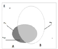
SIA can be presented as Figure 1 [21][22]. For binary variables, let 𝐸 be the population of 𝑛 objects or individuals described by a finite set of variables; 𝐴 (𝐵) be the subset of 𝐸
containing the object 𝑖 such that 𝐴(𝑖) = 𝑡𝑟𝑢𝑒 (B(𝑖) = 𝑡𝑟𝑢𝑒); sets 𝐴̅ , 𝐵̅ be the complement of set 𝐴 and 𝐵 respectively;
𝑛𝐴= 𝑐𝑎𝑟𝑑(𝐴), 𝑛𝐵= 𝑐𝑎𝑟𝑑(𝐵) be the cardinality of 𝐴 and 𝐵 respectively; 𝑛𝐴̅ = 𝑐𝑎𝑟𝑑( 𝐴̅) and 𝑛𝐵̅= 𝑐𝑎𝑟𝑑( 𝐵̅) be the cardinality of the set 𝐴̅ and the set 𝐵̅ respectively; and 𝑛𝐴𝐵̅ =
𝑐𝑎𝑟𝑑(𝐴 ∩ 𝐵̅) be the cardinality of the set 𝐴 ∩ 𝐵̅ containing the objects that satisfy the properties 𝐴 but does satisfy the properties 𝐵, 𝑛𝐴𝐵̅ is also called counter-example. For quantitative variables, 𝑛𝐴= ∑𝑛𝑖=1𝐴(𝑖), 𝑛𝐵̅= ∑𝑛𝑖=1(1 −
𝐵(𝑖)); 𝐴(𝑖)is the value given by object 𝑖 for set 𝐴; 𝐵(𝑖)is the value given by object 𝑖 for set B; and 𝑛𝐴𝐵̅ = ∑𝑛 (𝐴(𝑖) ∗ (1 −
𝑖=1
𝐵(𝑖)). The implication relationship between two variables 𝐴
and 𝐵(𝐴 → 𝐵 ) is presented by 4 parameters (𝑛, 𝑛𝐴, 𝑛𝐵, 𝑛𝐴𝐵̅).
Figure 1. The Venn diagram of the SIA presentation. For example, with two datasets of 9 objects described by 3 variables as Figure 2, the implication relationship between two variables (movies) Toy Story (1995) Star War (1997) is (9, 5.2, 7.8, 0.72) if variables are in the quantitative form and (9, 7, 8, 1) if variables are in the binary form.
Figure 2. Demonstration of statistical implication relationships: (𝐴 → 𝐵) = {
𝑛, 𝑛
𝐴, 𝑛
𝐵, 𝑛
𝐴𝐵̅}.2.2. Family of implication measures
The SIA’s measures are asymmetric. Unlike other data analysis methods, SIA is based on counter-examples, the smaller the counter-example is, the greater the degree of the implication relationship is and vice versa. Two important measures of SIA are the implication index and the implication intensity.
Implication intensity measure 𝜑(𝐴, 𝐵) of rule 𝐴 → 𝐵 is defined by (1) [22]:
𝜑(𝐴, 𝐵) =
{1 − ∑
𝜆𝑠 𝑠!𝑒
−𝜆 𝑛𝐴𝐵
𝑠=0 =
1
√2𝜋∫ 𝑒
−𝑡22𝑑𝑡 ∞
𝑞(𝐴,𝐵̅) , 𝑖𝑓 𝑛𝐵< 𝑛
0, 𝑜𝑡ℎ𝑒𝑟 𝑤𝑖𝑠𝑒
(1)
where 𝜆 =𝒏𝑨𝒏𝑩̅
𝒏 ; and 𝑞(𝐴, 𝐵̅), called the implication index, is defined by (2a) if data is binary form and (2b) if data is non-binary form.
When the approximation is justified (e.g. 𝜆 ≥ 4), 𝑞(𝐴, 𝐵̅)
is the approximation of the normal distribution 𝑁(0,1). The implication rule that A→B is admissible at the confidence level 𝛼 if and only if 𝜑(𝐴, 𝐵) ≥ 1 − 𝛼 [22].
𝑞(𝐴, 𝐵̅) =𝑛𝐴𝐵̅− 𝑛𝐴𝑛𝐵̅
𝑛
√𝑛𝐴𝑛𝐵̅
𝑛
(2a)
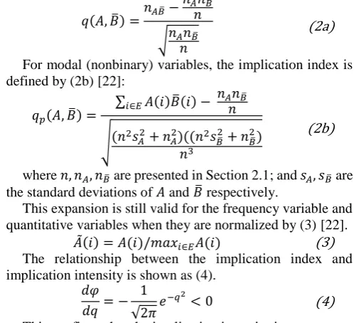
For modal (nonbinary) variables, the implication index is defined by (2b) [22]:
𝑞𝑝(𝐴, 𝐵̅) =
∑ 𝐴(𝑖)𝐵̅(𝑖) − 𝑛𝐴𝑛𝐵̅
𝑛
𝑖∈𝐸
√(𝑛2𝑠𝐴2+ 𝑛𝐴2)((𝑛2𝑠𝐵̅ 2+ 𝑛
𝐵̅ 2)
𝑛3
(2b)
where 𝑛, 𝑛𝐴, 𝑛𝐵̅ are presented in Section 2.1; and 𝑠𝐴, 𝑠𝐵̅ are the standard deviations of 𝐴 and 𝐵̅ respectively.
This expansion is still valid for the frequency variable and quantitative variables when they are normalized by (3) [22].
𝐴̃(𝑖) = 𝐴(𝑖)/𝑚𝑎𝑥𝑖∈𝐸𝐴(𝑖) (3)
The relationship between the implication index and implication intensity is shown as (4).
𝑑𝜑 𝑑𝑞= −
1
√2𝜋𝑒
−𝑞2
< 0 (4)
This confirms that the implication intensity increases as q decreases. The rate of increase is determined by (6), which allows a more rigorous study of the variability of φ.
2.3. Implication field
Let us consider 𝑛, 𝑛𝐴, 𝑛𝐵, 𝑛𝐴𝐵̅ as four real variables satisfying the inequalities [22]: 0 ≤ 𝑛𝐴≤ 𝑛𝐵; 𝑛𝐴𝐵̅ ≤ inf {𝑛𝐴, 𝑛𝐵} and
sup{𝑛𝐴, 𝑛𝐵} ≤ 𝑛. Let 𝑀 be the point in the four-dimensional space 𝑅4 whose coordinates are associated with A and B. The implication index 𝑞(𝐴, 𝐵̅) [21][22] is the function of four parameters 𝑞(𝑛, 𝑛𝐴, 𝑛𝐵, 𝑛𝐴𝐵̅). In this case, 𝑞 is a continuously differentiable function. The differential of q in Frechet’s geometry is expressed in the following way [21]:
𝑑𝑞 =𝛿𝑞 𝛿𝑛𝑑𝑛 +
𝛿𝑞 𝛿𝑛𝐴
𝑑𝑛𝐴+
𝛿𝑞 𝛿𝑛𝐵
𝑑𝑛𝐵+
𝛿𝑞 𝛿𝑛𝐴𝐵̅
𝑑𝑛𝐴𝐵̅ (5)
= 𝑑𝑀. 𝑔𝑟𝑎𝑑𝑞
where 𝑑𝑀 is the differential component vector of the instance variables and 𝑔𝑟𝑎𝑑. 𝑞 is the partial differential vector of the variables.
𝑞(𝐴, 𝐵̅) is a scalar field by applying the mapping from space 𝑅4 to space 𝑅. The vector 𝑔𝑟𝑎𝑑𝑞 containing the partial derivatives of 𝑞 for the variables 𝑛, 𝑛𝐴, 𝑛𝐵, 𝑛𝐴𝐵̅ is a gradient field. At each point of the gradient field, we observe an increase in the density of the implication in the space that changes under the influence of the transformation of one or more parameters. In this context, the gradient field is called the implication field. The mixed derivative event of each pair of variables [21], for example: 𝑛𝐵, 𝑛𝐴𝐵̅, is:
𝛿 𝛿𝑛𝐴𝐵̅
(𝛿𝑞 𝛿𝑛𝐵
) = 𝛿 𝛿𝑛𝐵
( 𝛿𝑞 𝛿𝑛𝐴𝐵̅
) (6)
A plane of equipotential in implication field is curved in
𝐸, an 4-dimensional space, that along which 𝑀 maintains the same value of potential of 𝑞. The plane of equipotential is orderly. The equation (7) of this curve is shown in [21]. The implication field is formed from a set of ordered equipotential
planes corresponding to the sequential successive values of q relative to the cardinalities (𝑛, 𝑛𝐴, 𝑛𝐵, 𝑛𝐴𝐵̅) that would be varied [21].
𝑞(𝐴, 𝐵̅) − 𝑛𝐴𝐵̅− 𝑛𝐴𝑛𝐵̅
𝑛
√𝑛𝐴𝑛𝐵̅
𝑛
= 0 (7)
3. Implication rules and association rules
A rule, denoted by 𝐴 → 𝐵, is a relation between a pair of sets
(𝐴, 𝐵). The examples (likelihood) of the rule are the objects identified by the antecedent 𝐴 and the consequence 𝐵, while the counter-examples (unlikelihood) of the rule are the objects identified by 𝐴 but negative 𝐵 as Table 1 shows the relationship of components of rule.
Table 1. Contingency table for rule 𝐴 → 𝐵 𝐵 𝐵̅ total
𝐴 𝑛𝐴𝐵 𝑛𝐴𝐵̅ 𝑛𝐴
𝐴̅ 𝑛𝐴̅𝐵 𝑛𝐴̅𝐵̅ 𝑛𝐴̅ total 𝑛𝐵 𝑛𝐵̅ 𝑛
A rule will have a better meaning when it has more examples and less counter-examples and vice versa. Likewise, a rule will be reinforced if the incremental component of the examples is faster than the incremental component of the counter-examples.
3.1. Association rules
An association rule is the simplification of a rule 𝐴 → 𝐵 in which 𝐴 and 𝐵 are two itemsets and 𝐴 ∩ 𝐵 = ∅. The association rule is modelled as a mathematical model of four parameters 𝑛, 𝑛𝐴, 𝑛𝐵 and a parameter of the distribution of both two variables such as 𝑛𝐴𝐵 [18]. Let ℛ𝐴𝑆𝑆 be a set of all association rules; ℛ𝐴𝑆𝑆 is presented by the following equation (8).
ℛ𝐴𝑆𝑆
=
{
(𝑛, 𝑛𝐴, 𝑛𝐵, 𝑛𝐴𝐵)
| |
𝑛𝐴≤ 𝑛, 𝑛𝐵≤ 𝑛,
𝑛𝐵≤ 𝑛,
max(0, 𝑛𝐴+ 𝑛𝐵− 𝑛)
≤ 𝑛𝐴𝐵≤ min(𝑛𝐴, 𝑛𝐵)
(𝑠𝑢𝑝𝑝𝑜𝑟𝑡 ≥ 𝑚𝑖𝑛𝑠𝑢𝑝, 𝑐𝑜𝑛𝑓𝑖𝑑𝑒𝑛𝑐𝑒 ≥ 𝑚𝑖𝑛𝑐𝑜𝑛𝑓)}
(8)
The algorithm, named as 𝐺ℛ𝐴𝑆𝑆, is used to generate the set of association rules (ℛ𝐴𝑆𝑆). In 𝐺ℛ𝐴𝑆𝑆, we use the Apriori algorithm [19][20] and the thresholds of support and confidence (𝑚𝑖𝑛𝑠𝑢𝑝 and 𝑚𝑖𝑛𝑐𝑜𝑛𝑓 respectively) to find the most useful rules. The main steps of this algorithm are:
Step 1: Finding the frequent itemsets (i.e. the sets of items that have minimum support)
Step 2: Using these frequent itemsets, the minimum confidence, and the minimum support to find rules
3.2. Implication rules
Implication association rule (referred to as implication rule) is also modelled by four parameters where the fourth one is the number of counter-examples 𝑛𝐴𝐵̅. Let ℛ𝐼𝑀𝑃 be a set of all implication rules, ℛ𝐼𝑀𝑃 is presented by the following equation (9).
ℛ𝐼𝑀𝑃
=
{
(𝑛, 𝑛𝐴, 𝑛𝐵, 𝑛𝐴𝐵̅)||
0 ≤ 𝑛𝐴≤ 𝑛𝐵≤ 𝑛 ,
0 ≤ 𝑛𝐴𝐵̅≤ 𝑛𝐵
(𝑠𝑢𝑝𝑝𝑜𝑟𝑡 ≥ 𝑚𝑖𝑛𝑠𝑢𝑝𝑝, 𝑐𝑜𝑛𝑓𝑖𝑑𝑒𝑛𝑐𝑒 ≥ 𝑚𝑖𝑛𝑐𝑜𝑛𝑓 𝑆𝐼𝐴 𝑚𝑒𝑎𝑠𝑢𝑟𝑒 ℜ 𝑡ℎ𝑟𝑒𝑠ℎ𝑜𝑙𝑑)}
(9)
Where ℜ is " ≤ " if the SIA measure belongs to the variance of the implication index measure, and ℜ is " ≥ " if the SIA measure belongs to the variance of the implication intensity measure. The SIA measure can be the implication index, the implication intensity, and their variations by the four parameters. In this paper, for the experiments, we use the variance of implication index by 𝑛𝐴𝐵̅.
SIA measures have the following properties [7] when compared to other probability and statistical measures:
- The implication index (and implication intensity) is an asymmetric and nonlinear statistical measure.
- The value of implication intensity increases with the size of the training set while other measures (support/confidence, lift, etc.) remain constant.
- The implication intensity reflects the way the human draws (removes) the previous statement. If a statement has strong implications, some counter-examples appear to be insufficient to change the implication of the rule. However, if the number of counterexamples appears more and more, the implication of the rule decreases; and eventually if the number of counter-examples is large enough, it will result in the elimination of the rule,
- The implication intensity is the good adaptation to noisy data, since a small number of counter-examples do not have the ability to invalidating the rule.
- The implication intensity does not allow the creation of rules such as 𝐴 → 𝐵 when 𝐵 is true for almost all examples of the training set whether 𝐴 is true or false. In that case, it is not surprising that the set with 𝐴 to be true is almost included in the set with 𝐵 to be true.
We developed the algorithm 𝐼𝑅𝐺 to generate the set of implication rules (ℛ𝐼𝑀𝑃). 𝐼𝑅𝐺 is similar to the algorithm used for association rules, but it also uses the statistical implication measures to constraint on rules. In this paper, we use the variance of implication index by 𝑛𝐴𝐵̅ (named as
𝑖𝑓𝑏𝑦𝐶𝑜𝑢𝑛𝑡𝐸𝑥𝑎𝑚) for the experiment.
Algorithm 1. IRG (Implication Rules Generator)
Input: a dataset; the thresholds of confidence, support and a SIA measure; type of data (binary/quantitative).
Output: Implication rule set.
Step 1: Constructing a measure of variance in the implication index in the implication field by the counter-example. The proposed measure, named as
𝑖𝑓𝑏𝑦𝐶𝑜𝑢𝑛𝑡𝐸𝑥𝑎𝑚, is calculated as the follow.
𝑖𝑓𝑏𝑦𝐶𝑜𝑢𝑛𝑡𝐸𝑥𝑎𝑚 = 𝑞(𝐴, 𝐵̅) + 1 √𝑛𝐴(𝑛 − 𝑛𝐵)
𝑛
Step 2: Generating the implication rules set from the dataset using a data mining algorithm (such as Apriori, Eclat, etc.) and the thresholds of support, confidence and
𝑖𝑓𝑏𝑦𝐶𝑜𝑢𝑛𝑡𝐸𝑥𝑎𝑚. Note that: if data is in binary form,
𝑞(𝐴, 𝐵̅) is computed by equation (2); if the data is in quantitative form, 𝑞(𝐴, 𝐵̅) is computed by equation (4) and (3).
Step 3: Presenting each implication rules by four values
𝑛, 𝑛𝐴, 𝑛𝐵, 𝑛𝐴𝐵̅ as well as its values according to the measures such as support, confidence, implication index, implication intensity, and 𝑖𝑓𝑏𝑦𝐶𝑜𝑢𝑛𝑡𝐸𝑥𝑎𝑚.
With the algorithm 𝐼𝑅𝐺, the generated implication rules will be more accurate because of the high examples (from support /confidence measures) and low counter-examples (from the statistical implication measure). This will be confirmed in the experimental section.
4. Recommendation
4.1. Based on association rules
The recommendation model based on the association rules
𝑀ℛ𝐴𝑆𝑆 consists of: a dataset; the type of data (binary or quantitative data); the thresholds of support and confidence; the algorithm for generating the set of association rules (creating model); the algorithm for predicting and displaying the recommendation result. If dataset is in the quantitative form, it has to be binarized. 𝑀ℛ𝐴𝑆𝑆 uses the algorithm 𝐺ℛ𝐴𝑆𝑆
(in Section 3) for generating the set of association rules ℛ𝐴𝑆𝑆.
𝑀ℛ𝐴𝑆𝑆 is presented as the following equation (10).
𝑀ℛ𝐴𝑆𝑆
=
{ 𝑋
| |
𝑑𝑎𝑡𝑎𝑠𝑒𝑡;
𝑡ℎ𝑟𝑒𝑠ℎ𝑜𝑙𝑑𝑠 𝑓𝑜𝑟 𝑠𝑢𝑝𝑝𝑜𝑟𝑡 𝑎𝑛𝑑 𝑐𝑜𝑛𝑓𝑖𝑑𝑒𝑛𝑐𝑒; 𝑡𝑦𝑝𝑒 𝑜𝑓 𝑑𝑎𝑡𝑎;
𝑎𝑙𝑔𝑜𝑟𝑖𝑡ℎ𝑚 𝐺ℛ𝐴𝑆𝑆 𝑓𝑜𝑟 𝑔𝑒𝑛𝑒𝑟𝑎𝑡𝑖𝑛𝑔 ℛ𝐴𝑆𝑆 ;
𝑎𝑙𝑔𝑜𝑟𝑖𝑡ℎ𝑚 𝑓𝑜𝑟 𝑝𝑟𝑒𝑑𝑖𝑐𝑡𝑖𝑛𝑔
𝑎𝑛𝑑 𝑑𝑖𝑠𝑝𝑙𝑎𝑦𝑖𝑛𝑔 𝑟𝑒𝑐𝑜𝑚𝑚𝑒𝑛𝑑𝑒𝑑 𝑟𝑒𝑠𝑢𝑙𝑡. } (10)
To predict and display the recommendation result to users, the recommendation model 𝑀ℛ𝐴𝑆𝑆 uses ℛ𝐴𝑆𝑆 and the
algorithm similar to the algorithm 𝑅𝐵𝑀𝐼𝑅 to be presented in Section 4.2.
4.2. Based on implication rules
Like 𝑀ℛ𝐴𝑆𝑆, the recommendation model based on implication
rule 𝑀ℛ𝐼𝑀𝑃 not only includes the components presented
quantitative dataset, and the algorithm 𝐼𝑅𝐺 in Section 3.2 for generating the set of implication rules.
Another difference from 𝑀ℛ𝐴𝑆𝑆, 𝑀ℛ𝐼𝑀𝑃 can use a set of recommendation models, each of which corresponds to a SIA measure such as implication index, the implication intensity, or the variance of those measures.
The recommendation model based on implication rules 𝑀ℛ𝐼𝑀𝑃 is presented as the following equation (11).
𝑀ℛ𝐼𝑀𝑃
=
{ 𝑋
| |
𝑑𝑎𝑡𝑎𝑠𝑒𝑡;
𝑡ℎ𝑟𝑒𝑠ℎ𝑜𝑙𝑑𝑠 𝑓𝑜𝑟 𝑠𝑢𝑝𝑝𝑜𝑟𝑡, 𝑐𝑜𝑛𝑓𝑖𝑑𝑒𝑛𝑐𝑒; 𝑆𝐼𝐴 𝑚𝑒𝑎𝑠𝑢𝑟𝑒 𝑎𝑛𝑑 𝑖𝑡𝑠 𝑡ℎ𝑟𝑒𝑠ℎ𝑜𝑙𝑑;
𝑡𝑦𝑝𝑒 𝑜𝑓 𝑑𝑎𝑡𝑎;
𝑎𝑙𝑔𝑜𝑟𝑖𝑡ℎ𝑚 𝐼𝑅𝐺 𝑓𝑜𝑟 𝑔𝑒𝑛𝑒𝑟𝑎𝑡𝑖𝑛𝑔 ℛ𝑖 ;
𝑎𝑙𝑔𝑜𝑟𝑖𝑡ℎ𝑚 𝑓𝑜𝑟 𝑝𝑒𝑑𝑖𝑐𝑡𝑖𝑛𝑔 𝑎𝑛𝑑 𝑑𝑖𝑠𝑝𝑙𝑎𝑦𝑖𝑛𝑔 𝑟𝑒𝑐𝑜𝑚𝑚𝑒𝑛𝑑𝑒𝑑 𝑟𝑒𝑠𝑢𝑙𝑡. }
(11)
The recommendation model 𝑀ℛ𝐼𝑀𝑃 is created by using the algorithm 𝑅𝐵𝑀𝐼𝑅. This algorithm is responsible for generating a set of implication rules and then recommending to users the appropriate items.
Algorithm 2. RBMIR (Recommendation by mining implication rules).
Input: a dataset; the thresholds of confidence, support and a SIA measure; type of data (binary/quantitative).
Output: 1 item or the list of top k items to be recommended to users.
Step 1: Calling the IRG algorithm for generating the set of implication rules.
Step 2: Predicting and returning the recommendation result (1 item or k items) to users.
4.3. Evaluation of recommendation
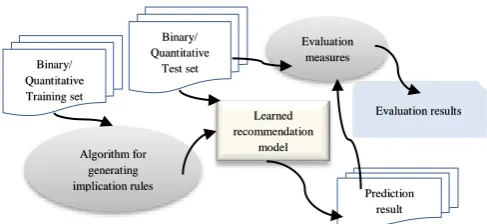
Figure 3 illustrates the workflow to be used for evaluating the proposed systems. Firstly, the training set is used by the proposed algorithm (𝐺ℛ𝐴𝑆𝑆 or 𝐼𝑅𝐺) to create a set of rules (a
learned recommendation model). Secondly, that model uses the test set with known labels to make the prediction. Lastly, the prediction result and the test set with unknown labels are then compared by some of measures to generate the evaluation results.
To evaluate the accuracy of the list of useful items recommended to a user, we often compare the predicted items with the items already preferred by that user. Each item can be classified as Positive (TP), False-Positive (FP), True-Negative (TN), or False-True-Negative (FN) [8][23][28] as shown in Table 2. This matrix is often referred to as the confusion matrix.
*https://kdd.ics.uci.edu/databases/msweb/msweb.html
Figure 3. Recommendation evaluation process.
Table 2. Confusion Matrix for recommendation systems Recommended Not Recommended Purchased True Positive (TP) False Negative (FN)
Not
purchased False Positive (FP) True Negative (TN) The measures such as TPR (True Positive Rate), FPR (False Positive Rate), precision, recall, and F_score (F1) [8][28][23] are used to evaluate the use of predictions. TPR is the percentage of purchased items that have been recommended. It is the ratio between the number of TP and the number of purchased items (TP + FN). FPR is the percentage of no purchased items that have been recommended. It is the ratio between the number of FP and the number of non-purchased items (FP + TN). The equations of precision, recall and F1 are shown in the following equations (12), (13) and (14) respectively.
𝑝𝑟𝑒𝑐𝑖𝑠𝑖𝑜𝑛 = 𝑇𝑃
𝑇𝑃 + 𝐹𝑃 (12)
𝑟𝑒𝑐𝑎𝑙𝑙 = TP
𝑇𝑃 + 𝐹𝑁 (13)
𝐹1 =2 × 𝑃𝑟𝑒𝑐𝑖𝑠𝑖𝑜𝑛 × 𝑅𝑒𝑐𝑎𝑙𝑙
𝑃𝑟𝑒𝑐𝑖𝑠𝑖𝑜𝑛 + 𝑅𝑒𝑐𝑎𝑙𝑙 (14)
5. Experiment
The purpose of this experiment is to evaluate the performance and accuracy of the recommendation model based on implication rules and those of the recommendation model based on association rules (traditional ARM models). The SIA measure used by the experiment of this paper is the variation of the implication index in the implication field.
5.1. Data
We conduct the experiment on both binary dataset (MSWeb*)
and quantitative dataset (Movielens†). MovieLens collected by GroupLens is of 100,000 ratings given for 1682 films by 943 users. The ratings range from 1 (the lowest) to 5 (the highest). MSWeb is collected by listing all Vroots (the areas of the web site www.microsoft.com) that are visited by 38000
† https://grouplens.org/datasets/movielens/ Algorithm for
generating implication rules
Learned recommendation
model Binary/
Quantitative Training set
Binary/ Quantitative
Test set
Prediction result Evaluation results Evaluation
anonymous, randomly-selected users in one-week timeframe. The datasets are pre-processed by normalizing and selecting relevant data to limit the bias, thereby to avoid overfitting problems as well as to get better accuracy.
We conduct the experiment in k-fold cross validation mode, with k=5. The steps of this mode is the follows: (1) Splitting the dataset (Movielens or MSWeb) into 5 equal sized parts; (2) Training on four parts and evaluating on the remaining one; (3) Repeating the second step by using different parts as the test set (the grey part):
Part 1 Part 2 Part 3 Part 4 Part 5 𝐴𝑐𝑐𝑢𝑟𝑎𝑐𝑦1 Part 1 Part 2 Part 3 Part 4 Part 5 𝐴𝑐𝑐𝑢𝑟𝑎𝑐𝑦2 Part 1 Part 2 Part 3 Part 4 Part 5 𝐴𝑐𝑐𝑢𝑟𝑎𝑐𝑦3 Part 1 Part 2 Part 3 Part 4 Part 5 𝐴𝑐𝑐𝑢𝑟𝑎𝑐𝑦4 Part 1 Part 2 Part 3 Part 4 Part 5 𝐴𝑐𝑐𝑢𝑟𝑎𝑐𝑦5 The quality of recommendation model is the average of 5 evaluations.
𝐴𝑐𝑐𝑢𝑟𝑎𝑐𝑦 = 𝐴𝑐𝑐𝑢𝑟𝑎𝑐𝑦1+ … + 𝐴𝑐𝑐𝑢𝑟𝑎𝑐𝑦5 5
5.2. Tools
We develop a tool in the R language. The tool consists of the proposed recommendation models and the utility functions to be used for this experiment.
5.3. Scenario
1: association rules vs
implication rules on binary dataset
This scenario evaluates the accuracy of two recommendation systems IFARRS (based-on implication rules) and ARRS (based-on association rules) on binary dataset. IFARRS uses the recommendation model based on implication rules whereas ARRS uses the recommendation model based on association rules. In both systems, the number of items to be recommended to a user is 1, 5, 10, 20 and 25; and the thresholds of support and confidence are 0.1 and 0.3 respectively.
The comparison result is presented in Table 3 and Figure 4. They show that the precision, recall and the reconciliation between precision and recall (F1) of IFARRS is higher than those of ARRS as well as the false positive rate of IFARRS is lower than that of ARRS. However, the recall of IFARRS is lower than that of ARRS. Therefore, for systems where the precision, recall or F1 is important, we should use the model based on implication rules to make the recommendation.
Table 3. Experimental results accuracy of two models on binary dataset.
Precision Recall F1 TPR FPR
ARRS Model
1 0.328 0.069243 0.338381 0.069243 0.003929
5 0.295771 0.303008 0.344725 0.303008 0.020587
10 0.248114 0.493032 0.32858 0.493032 0.043966
20 0.170629 0.666089 0.264644 0.666089 0.097064
25 0.147383 0.713444 0.238388 0.713444 0.124756
IFARRS Model
1 0.476525 0.101835 0.342267 0.101835 0.00305
5 0.358738 0.364551 0.386516 0.364551 0.018452
10 0.283955 0.518019 0.365517 0.518019 0.038844
20 0.257943 0.609764 0.355118 0.609764 0.055464
25 0.257419 0.611912 0.355015 0.611912 0.056025
Figure 4. The ROC and Precision/Recall Curves of ARRS and IFARRS on MSWeb dataset
5.4. Scenario
2: association rules vs
implication rules on quantitative dataset
This scenario is similar to Scenario 1, but it uses the quantitative dataset MovieLens. In both systems IFARRS and ARRS, the number of items to be recommended to a user is 1, 5, 10, 20 and 25; and the thresholds of support and confidence are 0.1 and 0.3 respectively.
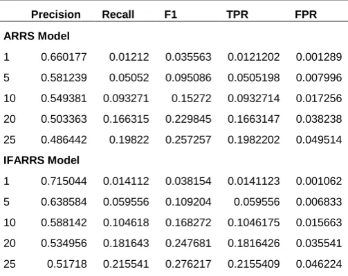
The results in Table 4 and Figure 5 show that the accuracy (precision, recall, F1) of IFARRS is higher than that of ARRS; and the false positive rate of IFARRS is lower than that of ARRS. Therefore, for the quantitative datasets, we should use the implication rules based model to build the recommendation systems.
Table 4. Experimental results accuracy of two models on quantitative dataset.
Precision Recall F1 TPR FPR
ARRS Model
1 0.660177 0.01212 0.035563 0.0121202 0.001289
5 0.581239 0.05052 0.095086 0.0505198 0.007996
10 0.549381 0.093271 0.15272 0.0932714 0.017256
20 0.503363 0.166315 0.229845 0.1663147 0.038238
25 0.486442 0.19822 0.257257 0.1982202 0.049514
IFARRS Model
1 0.715044 0.014112 0.038154 0.0141123 0.001062
5 0.638584 0.059556 0.109204 0.059556 0.006833
10 0.588142 0.104618 0.168272 0.1046175 0.015663
20 0.534956 0.181643 0.247681 0.1816426 0.035541
Figure 5. The ROC and Precision/recall Curve of ARRS and IFARRS models on Movielens dataset.
5.5. Scenario 3: the performance and
recommendation time
This scenario is used for evaluating the performance (in terms of the size of the rule set) and the recommendation time (in term of the modelling time and the predictive time) of two recommendation systems IFARRS and ARRS.
Table 5 shows the result of both systems on MovieLens when the number of items to be recommended to a user is 5. The ratio between (the modelling time, the predicting time, the size of rule set) of IFARRS and those of ARRS is (0.4657, 0.6280, 0.0912) respectively. This demonstrates that the IFARRS on quantitative rules produces the better rule enforcement, has the faster recommendation time. This is result of the combination of the support and confidence measures for finding the rules with likelihood and the
ifbyCountExam measure for filtering the rules with unlikelihood.
Table 5. Comparison of training time, predicting time and size of the rule set generated by the two models
No Name Modelling
time
Predicting time
Size of rule
1 ARRS
model 42.12367 10.58138 688536
2 IFARRS
model 19.61867 6.645375 62796
6. Conclusion
The statistical implication analysis theory can be applied for building recommendation systems where the relationships among properties can be considered as implication rules. This paper proposes the implication rules based recommendation model on both binary and quantitative datasets. For the experiment, the proposed model uses the variance of the implication index in the implication field named as
𝑖𝑓𝑏𝑦𝐶𝑜𝑢𝑛𝑡𝐸𝑥𝑎𝑚. The proposed model is compared with the association rule based recommendation model. The experimental results show that the proposed model increases the effectiveness of the recommendations: increasing the accuracy of recommended result, expanding the recommendations for quantitative data sets, as well as significantly reducing the number of rules to make the system faster and more efficient.
References
[1] Adomavicius Gediminas, Tuzhilin Alexander, (2005) Toward the Next Generation of Recommender Systems: A Survey of the State-of-the-Art and Possible Extensions, IEEE transactions on Knowledge and Data engineering, Vol.17 No.6, pp. 734 – 749.
[2] Ahmed Mohammed K. Alsalama (2015), A Hybrid Recommendation System Based On Association Rules, International Science Index, Computer and Information Engineering Vol:9, No:1, 2015 waset.org/Publication/10000147
[3] Andi Asrafiani Arafah, Imam Mukhlash (2015), The Application of Fuzzy Association Rule on Co-Movement Analyze of Indonesian Stock Price, International Conference on Computer Science and Computational Intelligence (ICCSCI 2015), Procedia Computer Science 59 pp. 235 – 243.
[4] Breese, J.S. and D. Heckerman, 1998. Empirical analysis of predictive algorithms for collaborative filtering. Morgan Kaufmann, pp. 43–52.
[5] Dhrubajit Adhikary, Swarup Roy (2015), Trends in Quantitative Association Rule Mining techniques, 2015 IEEE 2nd International Conference on Recent Trends in Information Systems (ReTIS). DOI: 10.1109/ReTIS.2015.7232865.
[6] Francesco Ricci, Lior Rokach and Bracha Shapira (2011): Introduction to Recommender Systems
Handbook, Springer-Verlag and Business Media LLC, pp.1-35, (2011).
[7] Guillaume S., Guillet F., Philipp6 J. (1998): Contribution of the integration of intensity of implication into the algorithm proposed by Agrawal, EMCSR'98, Vienna, vol. 2, pp. 805-810.
[8] Herlocker J.L et al, 2004. Evaluating collaborative filtering recommender systems. ACM Trans. Inf. Syst., vol. 22, no. 1, pp. 5–53
[9] Hoang Tan Nguyen, Hung Huu Huynh and Hiep Xuan Huynh (2018), Collaborative filtering recommendation with threshold value of the equipotential plane in implication field, the 2nd International Conference on Machine learning and Soft computing (ICMLSC2018); Phu Quoc island, Vietnam, ISBN: 978-1-4503-6336-5 pp.39-44.
[10] Hoang Tan Nguyen, Hung Huu Huynh and Hiep Xuan Huynh (2018), Collaborative Filtering Recommendation in the Implication Field, International Journal of Machine Learning and Computing, Volume 8 Number 3 (Jun. 2018), pp 214-222
[11] Hoang Tan Nguyen, Hung Huu Huynh and Hiep Xuan Huynh (2017), The Collaborative filtering recommendation based-on the variance implication index by the counter-example in the implication field. Proceedings of the XXI National Conference “Some selected issues of information and communications technology (@ ‘2017). Quy Nhon, VietNam, pp. 372-379. (in Vietnamese)
of implication index in statistical implication field, Proceedings of the X National Conference on Fundamental and Applied IT Re-search (FAIR’17); Da Nang,. ISBN: 978-604-913-614-6, pp. 938-950 (in Vietnamese).
[13] Lan Phan Phương, Trang Trần Uyên, Hưng,Huỳnh Hữu, Hiệp , Huỳnh Xuân,(2016) User-based collaborative filtering recommendation using statistical implication cohesion measure. Proceedings of the VIII National Conference on Fundamental and Applied IT Research (FAIR’15); Cần Thơ, 2016, (in Vietnamese). [14] Lan Phan Phương, Hưng,Huỳnh Hữu, Hiệp , Huỳnh Xuân,(2018) Recommendation using Rule based Implicative Rating Measure, International Journal of Advanced Computer Science and Applications (IJACSA).
[15] Lan Phan Phương, Hưng,Huỳnh Hữu, Hiệp , Huỳnh Xuân,(2018) Recommender systems based-on implication intensity and contribution measure, , Proceedings of the X National Conference on Fundamental and Applied IT Re-search (FAIR’17); Da Nang,. ISBN: 978-604-913-614-6, (in Vietnamese). [16] Masakazu Seno and George Karypis (2005). Finding
frequent itemsets using length-decreasing support constraint. Data Mining and Knowledge Discovery, 10:pp.197–228.
[17] Nghia Quoc Phan, Ky Minh Nguyen, Hoang Tan Nguyen, Hiep Xuan Huynh, Recommender systems based approach combining association rule and implicative statistical measure, Proceedings of the VIII National Conference on Fundamental and Applied IT Research (FAIR’15); Ha Noi, 2015. (in Vietnamese). [18] Piatetsky-Shapiro, G. (1991). Discovery, analysis, and
presentation of strong rules. In Knowledge Discovery in Databases, (pp. 229–248). AAAI/ MIT Press. [19] Rakesh Agrawal, Imielinski, T., & Swami, T. (1993).
Mining association rules between sets of items in large databases. In Proceedings of ACM SIGMOD international conference on management of data (SIGMOD’93) (pp. 207–216)
[20] Rakesh Agrawal and Ramakrishnan Srikant Fast algorithms for mining association rules. Proceedings of the 20th International Conference on Very Large Data Bases, VLDB, pages 487-499, Santiago, Chile, September 1994
[21] Régis Gras, Pascale Kuntz et Nicolas Greffard, (2015) Notion de champ implicatif en analyse statistique implicative, VIII Colloque International, A.S.I. Analyse Statistique Implicative - Statistical Implicative Analysis Radès (Tunisie) - Novembre 2015, 29-46. [22] Régis Gras, Einoshin Suzuki Fabrice Guillet, Filippo
Spagnolo (Eds.) (2009): Statistical Implicative Analysis, Theory and Application. Springer Verlag Berlin Heidelberg.
[23] Sarwar, B and G. Karypis, 2000. Analysis of recommendation algorithms for ecommerce. EC ’00. USA: ACM, pp. 158–167
[24] Sergey Brin, Rajeev Motwani, Jeffrey D. Ullman, and Shalom Tsur (1997). Dynamic itemset counting and implication rules for market basket data. In SIGMOD 1997, Proceedings ACM SIGMOD International Conference on Management of Data, Tucson, Arizona, USA, pp.255–264,
[25] Timur Osadchiy, Ivan Poliakov, Patrick Olivier, Maisie Rowland, Emma Foster (2018), Recommender system
based on pairwise association rules,
Expert Systems With Applications 115 535–542. https://doi.org/10.1016/j.eswa.2018.07.077
[26] Tzung Pei Hong, Chang Sheng Kuo, Sheng Chai Chi, (2001) Trade-off between computation time and number of rules for fuzzy mining from quantitative data, International journal of Uncertainty, Fuzziness and Knowledge-Based Systems Vol.9, No.5, pp.587-604.
[27] Tzung-Pei Hong, Chun-Hao Chen, Yeong-Chyi Lee, and Yu-Lung Wu. (2008), Genetic-Fuzzy Data Mining With Divide-and-Conquer Strategy, IEEE TRANSACTIONS ON EVOLUTIONARY COMPUTATION, VOL. 12, NO. 2, APRIL 2008. [28] Yeong, et al, 2005. Mining changes in customer buying
behavior for collaborative recommendations. Expert Syst. Appl. 28, 2 (February 2005), 359-369. DOI=10.1016/j.eswa.2004.10.015
http://dx.doi.org/10.1016/j.eswa.2004.10.015