PROBABILITY BASED OPTIMAL ENERGY CONSUMPTION IN WSN FOR DIFFERENT STRUCTURES

PROBABILITY BASED OPTIMAL ENERGY

CONSUMPTION IN WSN FOR DIFFERENT

STRUCTURES

1

Ram Krishna Sharma,

Kamlesh Kumar Mishra

1

Department of Electronics & Communication Engineering, UIT, Allahabad (India)

2

Assistant Professor, Department of Electronics & Communication Engineering, UIT, Allahabad (India)

ABSTRACT

Scheduled Rendezvous schemes have a disadvantage that some nodes can be active while data are not present. On-demand schemes have advantage that nodes will be active only for data is present and nodes want to communicate to each other necessarily. The power management approach using LEACH is applied which is specifically on-demand MAC protocol with low duty cycle. Assuming LEACH uses Direct Transmission protocol and assuming identical expected distance for all cluster Heads from the sink and for all leaf nodes from their cluster heads, Decentralized MAC using sleep-awake protocol is applied to reduce the energy consumption and then we analyze and calculate probability based energy consumption per node averagely. The analysis is presented for small hexagonal networks. We also analyze average Energy consumption and network life time for different shapes of WSN geographical infrastructure.

Keywords: Squared Structure, LEACH, Reduced Energy Consumption

I INTRODUCTION

II RELATED WORKS

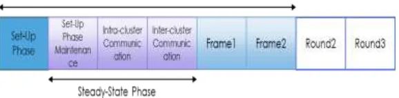
LEACH incorporates randomized rotation of the high-energy cluster head position among the sensors to avoid draining the battery of any one sensor in the network. In this way, the energy load of being a cluster head is evenly distributed among the nodes. The operation of LEACH is divided into rounds [2, 3 and 7] and each period consists of a set-up phase and a steady-state phase. During the setup phase, nodes communicate with short messages and are organized into clusters with some nodes selected as cluster heads. After the set-up phase, each cluster head sets up TDMA schedules for all leaf nodes in its cluster. Leaf nodes send any data to the cluster heads according to the TDMA schedule. [4]

Fig. 1: Description of a round as well protocols.

Each round consists of setup phase (formation of new cluster heads), steady-state phase (an intra-cluster communication phase and an inter cluster communication phase) and frame transmission which is data to be sent. [4, 8] A number of schemes to prolong the lifetime of sensor networks have been proposed in different literatures. However, appropriate cluster head selection mechanisms are required to reduce the energy consumption and enhance the lifetime of the network. Each node computes the quotient of its own energy level and the aggregate energy remaining in the network. With this value each node decides if it becomes cluster head for this round or not. Nodes with higher power are more likely to become cluster heads than nodes with lower power. The problem with this scheme is that each node has to estimate the remaining energy in the network which requires additional communication with the sink node and other nodes. [5] The optimal number of cluster-head selection for optimal probability of being cluster head to prolong the lifetime of WSNs based on LEACH architecture is calculated for a squared structure of a wireless sensor network. [2] In this paper, we propose an optimal cluster head selection algorithm to prolong the lifetime of WSNs based on the LEACH architecture for hexagonal field of a wireless sensor network.

III PROTOCOL DESCRIPTION AND ANALYSIS

There are certain problems while using a normal LEACH. [8]Two of them are,

3.1 Since cluster heads spend more energy than leaf nodes, it is quite important to reselect cluster heads periodically.

3.2 The TDMA mechanism which is used by LEACH for intra-cluster communication does not scale when the number of nodes increases.

IV ASSUMPTIONS FOR SELECTION OF CLUSTER-HEADS

There are two categories of nodes: First is Cluster Head nodes and the next is Non-cluster Head nodes or Leaf Nodes. In a cluster, there is a cluster head and remaining are Non-cluster Head nodes. There are some assumptions for the selection of a cluster head in a cluster: [1, 7]

4.1.All the non-cluster head nodes have data to send in a cluster. It means intra-communication phase is such a long so that every non-cluster head node can have data to send.

4.2.Inter-communication phase is such a long so that every cluster head can have data to send.

4.3.Sink is assumed to be stationary and reachable to all the nodes in the network. Similarly cluster heads are reachable to the non-cluster head nodes in a cluster.

4.4.The cluster heads perform data aggregation and compression before transmitting to the sink.

V CALCULATION OF ENERGY CONSUMPTION

We consider a network area

2 3 3 D_H2

meters for hexagonal network with N sensor nodes randomly distributed with uniform distribution. The distance of the cluster heads to the sink is denoted by d_inter and the distance between the

non-cluster head nodes in a non-cluster and their non-cluster head is denoted byd_intra. Let probability that data is available at a node

in a cluster isp_a. b_data , b_inter and b_intra are the message bits for transmission, payload for inter-communication and

payload for intra-communication simultaneously.

We assume that the radio dissipates Eelec J/bit to run the transmitter or receiver circuit and Eamp J/m

2

-bit for the transmitter amplifier to achieve an acceptable signal to noise ratio. Then Energy consumption due to transmission of b bit data and reception of b bit data are respectively given below.

 

   1

, 2        elec Rx amp elec Tx bE b E d bE bE d b E

Hence, energy consumption by a leaf node

 , _int  int (1 ) int _  2

                            T T E p b T T E d b E p

E_{NCH a Tx data ra Rx} ra _{data a Rx} ra

Where T= transmission and reception time, Tinter = the time devoted for inter cluster communications and Tint ra= the

time devoted for intra cluster communications. Where T  TinterandT  Tint ra .

Similarly energy consumption by a Cluster Head node can be given as

 , _int  int (1 ) int int _  3

                                         T T E T T E p b T T E d b E p

E_{CH ha Tx data er Rx} er _{data ha Rx} er _Rx ra

N E p N NpE TotalNodes E

E_avg  Total  CH  (1 ) NCH

1  _NCH  4

CH

avg pE p E

E   

Assuming T_inter and T_intra are equal, using b_inter and b_intra using relation between T_inter and b_inter as well as T_{int ra}

and bint ra and calculating phausingpa , the average energy can be calculated from equations (1), (2), (3) and (4) as

 









amp data

avg b E p p d p p d E pb b

E       

And k (cluster size) can be calculated as

p k  1

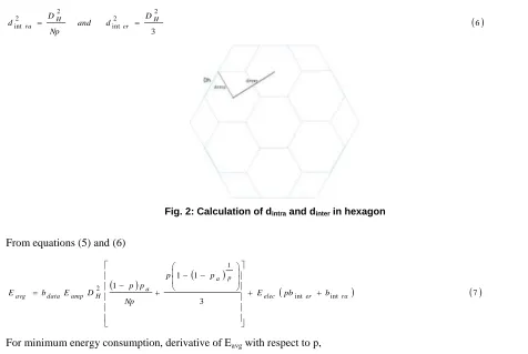
Now d_inter and d_intra can be calculated by using Voronoi Tessellation. Hence assuming d_inter as expected distance

between cluster heads and sink node and dintra as expected distance between cluster head and non-cluster head nodes,

using Voronoi Tessellation,

 6 3 2 2 int 2 2 int H er H ra D d and Np D

d  

Fig. 2: Calculation of dintra and dinter in hexagon

From equations (5) and (6)

    _{   } 7 3 1 1 1 int int 1 2 ra er elec p a a H amp data

avg E pb b

p p Np p p D E b

E  

                          

For minimum energy consumption, derivative of Eavg with respect to p,

0 

dp dE_avg

And assuming all the nodes have data to be sent, we get an optimal value of probability for being a cluster head





Hence,





3

3 3

int int 1 1

1 2

1 2

min

, elec opt er ra

opt opt opt

H amp data

avg E p b b

Np p Np

D E b

E  

   

  

 _{ }



VI VERIFICATION OF RESULT

Let, Eamp =100x10

-12 _J/m2_-bits,

elec

E =50x10-9 J/bits, N=1000 nodes, b_data =3000 bits/sec, b_inter =3000bits

D=100 meter for square region and DH is the dimension of hexagon of area D2 =10000 m2. Hence we get, popt1= 0.045

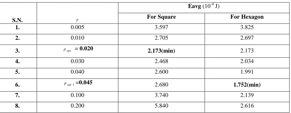
Hence energy consumption at p_opt and at different values of p is shown below in table. The analysis shows that when

we use Hexagon arrangement of a cluster in hexagonal area same as the area of square then energy consumption per node is very less for same number of nodes. The analysis is done by using MATLAB. This analysis also shows the result that increment in energy consumption is very less after the optimal probability for being a cluster head. This analysis can also be verified by the Tables (1 and 2) and figures (3 and 4) shown.

TABLE 1. Average Energy Consumption v/s Probability (N=1000)

S.N. p

Eavg (10-4 J)

For Square For Hexagon

1. 0.005 3.597 3.825

2. 0.010 2.705 2.697

3. popt = 0.020 2.173(min) 2.173

4. 0.030 2.468 2.034

5. 0.040 2.600 1.991

6. popt1=0.045 2.680 1.752(min)

7. 0.100 3.740 2.139

8. 0.200 5.840 2.616

TABLE 2. Average Energy Consumption v/s Number of Nodes

S.N. N

Square Region Hexagon Region

Popt Eavg (in J) Popt1 Eavg (in J)

1. 200 0.047 2.873x10-4 0.097 2.253x10-4

2. 300 0.039 2.626x10-4 0.079 2.120x10-4

3. 500 0.030 2.376x10-4 0.062 1.985x10-4

4. 600 0.027 2.301x10-4 0.056 1.944x10-4

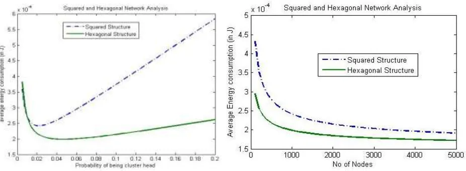
It is clear from the above two tables that the energy consumption per node is reduced by using the hexagonal structure in wireless sensor network. The tables also show that the average energy consumption reduces as number of nodes in a certain area (node density) increases.

Analysis also shows that average energy consumption per node is lesser for hexagonal network. The plot (using MATLAB 2011b) verifies the result in Figure 3. Average energy consumption per node per node decreases as number of nodes increases. The plot verifies the result in Figure 4.

Fig. 3: Variation in Probability Fig. 4: Variation in Number of Nodes

VII CONCLUSION AND FUTURE SCOPE

The analysis shows that the average energy consumption in different wireless sensor networks of same area having equal number of sensor nodes can be different for different structures. The new structure (Hexagonal) used in this analysis has provided a reduced average energy consumption over the previous structure (Squared). This analysis has its future scope that other structures of wireless sensor networks can be analyzed against the average energy consumption of the network for reduction in energy consumption.

VIII ACKNOWLEDGEMENT

REFERENCES

[1]Wang Jianguo, Wang Zhongsheng, Shi Fei, Song Guohua, “Research on Routing Algorithm for Wireless Sensor Network Based on Energy Balance”, American Journal of Engineering and Technology Research Vol. 11, No.9, 2011.

[2]Xiaoyan Cui, “Research and Improvement of LEACH Protocol in Wireless Sensor Networks”, IEEE 2007 International Symposium on Microwave, Antenna, Propagation, and EMC Technologies For Wireless Communications

[3]Wendi B. Heinzelman, Anantha P. Chandrakasan, Hari Balakrishnan, “An Application-Specific Protocol Architecture for Wireless Microsensor Networks”, IEEE transactions on wireless communication, Vol. 1, No. 4, October 2002

[4]W. Ye, J. Heidemann and D. Estrin, “An Energy efficient MAC Protocol for Wireless Sensor Networks,” Proceedings of IEEE INFOCOM, 2001.

[5]Hu Junping, Jin Yuhui, Dou Liang,” A Time-based Cluster-Head Selection Algorithm for LEACH”, 978-1-4244-2703-1/08/$25.00 ©2008 IEEE

[6]Wendi Rabiner Heinzelman, Anantha Chandrakasan, and Hari Balakrishnan, “Energy-Efficient Communication Protocol for Wireless Microsensor Networks”, 2000 IEEE, Hawaii International Conference on System Sciences, January 4-7, 2000, Maui, Hawaii.

[7]Giuseppe Anastasi, Marco Conti, Mario Di Francesco, Andrea Passarella, “Energy Conservation in Wireless Sensor Networks: a Survey”, Department of Information Engineering, University of Pisa, Italy, Institute for Informatics and Telematics (IIT), National Research Council (CNR), Italy