432 | P a g e
AN IMPROVED METHOD OF PID CONTROLLER
TUNING FOR UNSTABLE SYSTEM WITH DEAD TIME
USING IMPULSE INPUT
Nidhi Yadav
1,
*Mr. S.K. Sharma
21, 2
Chemical Engineering Department, DCRUST Murthal, (India)
ABSTRACT
Proportional-integral-derivative (PID) controllers tuning methods reported based on the approximate plant models derived from the step response. In this paper, an improved method proposed which based on the direct synthesis method approach (Maclaurin Series) using impulse input instead of step input. For unstable first-order process with dead time (FOUPDT) and second order process with dead time (SOUPDT) system in second order system there two conditions are considered i.e. One unstable and One stable Pole, Two Unstable Poles. Improved method is compare with other available methods for verifying the improved method. Controller tuning methods are compared each other i.e. Ziegler-Nichols method (Z-N) [6], C.T. Huang and Y.S. Lin (H-L) [2], Shamsuzzoha and Lee (S-L) [1], Q. Wang, C. Lu and W. Pan (W-P) [4], Poulin and Pomerleau (P-P) [3], Tayrus and Luyben (T-L) [10], Yongho Lee, Jeongesko Lee, Sunwon Park [7]. Two analysis (Time domain specification and Time integral performance) have observe for these controller tuning methods for finding the response of given methods, on the basis of these analysis methods are compared for FOUPDT and SOUPDT.
Keywords: Dead time, FOUPDT, IAE, ISE, ITAE, PID controller, SOUPDT, Tuning, Time constant
I. INTRODUCTION
Proportional-integral-derivative (PID) controllers have been widely used in process industries for decades. The
major reasons for their wide acceptance in industries are their ability to control most of the processes,
well-understood control action and ease of implementation. Proportional-integral-derivative (PID) controller has
remained as commonly used controllers in industrial process control for 50 yr. even though great progress in control
theory design and tuning of PID controllers has been the subject of many researchers working in this field. This
because it has a simple structure and is easily understood by the control engineers (Luyben, 1990). As early as 1942,
Ziegler and Nichols (1942) proposed the first PID tuning method. It is still widely used in practice at present. While
high performance is always, the design target in industrial control applications and the Ziegler-Nichols method is
insufficient in such applications. A survey of [8] Desborough and Miller reported that more than 97% of the
regulatory controllers utilize the PI/PID algorithm. The PI/PID controllers have only few adjustable parameters, and
are difficult to tune properly in real processes. Many researchers have provided PID controller settings for various
process models and different performance criteria. All the tuning relations reported in literature based on the
approximate plant models derived from the step input of the plant in this paper an improved method is developed for
PID controller tuning which is based on the direct synthesis method (in which mathematical approach comes) by
433 | P a g e
has a strong nonlinearity due to the heat generation term in the energy balance. In general, transfer function unstable
processes are FOUPDT (Huang & Lin, 1995) [2] and SOUPDT having two different case; i) One unstable and One
stable pole, ii) Two unstable poles (Yongho & Jeongesko Lee, 1999) [7] are given below,
FOUPDT:
-θs
Ke G(s) =
(τs-1)
SOUPDT: i) One unstable and one stable pole:
-θs
1 2
Ke G(s) =
(τ s-1)(τ s+1)
ii) Two unstable poles:
-θs
1 2
Ke G(s) =
(τ s-1)(τ s-1)
In this paper, comparison of Ziegler-Nichols (1942) [6], C.T. Huang and Y.S. Lin (1995) [2], Shamsuzzoha and Lee
(2007) [1], Q. Wang, C. Lu and W. Pan (2015) [4] methods are used for FOUPDT. Ziegler-Nichols (1942) [6],
Tayrus and Luyben (1958) [10], C.T. Huang and Y.S. Lin (1995) [2], Poulin and Pomerleau (1996) [3] are used for
SOUPDT (One unstable and One stable pole) and Yongho & Jeongesko Lee (1999) are used for (Two unstable
poles). Time domain specification and Time integral performance of all methods are use for finding the best
controller tuning method which gives better and higher stability for the process system. MATLAB 7.8 (2009),
controller-designing software used in this work. Fig.1 classical feedback process diagram
II. DEVELOPMENT OF PID CONTROLLER SETTINGS
A PID controller designated by,
P D
I
1 G(s) = K (1+ +τ s)
τ s ……….. (A)
Where, KP= Proportional Gain, τI= Integral constant, τD= Derivative constant
For the best performance of the system, need to adjust these three parameters called controller tuning.
Fig.1 Classical Feedback Diagram
Consider the block diagram of feedback control system shown in Fig.1. The objective is to design a PID controller,
C
G (s)
of Fig. 1 that will give the desired closed-loop response, Y/R, as specified byG (s)
D which described byeither FOUPDT or SOUPDT model. The actual closed-loop response of the control system in Fig.1 is denoted and
given by
G (s)
A is,C P
A
C P
G (s)G (s) Y(s)
G (s) = =
R(s) 1+G (s)G (s)
…………. (1)
Both G (s) and A G (s)d can represent by Maclaurin series expansion in
at
s = 0
2 3
' '' '''
A A A A A
s s
G (s) = G (0)+sG (0)+ G (0)+ G (0)+...
434 | P a g e
2 3
' '' '''
d d d d d
s s
G (s) = G (0)+sG (0)+ G (0)+ G (0)+...
2! 3! …………. (3)
Where the prime indicates the derivative with respect to s. Note that truncation of the series up to third-order term is
sufficient to setup three independent equations to determine the PID controller parameters. For an ideal controller,
the closed-loop response of the actual system results in the desired closed-loop response. Then by comparison, of (2)
and (3) we have,
A d
G (0) = G (0) ………. (4.1)
' '
A d
G (0) = G (0) ………. (4.2)
'' ''
A d
G (0) = G (0) ………. (4.3)
''' '''
A d
G (0) = G (0) ………. (4.4)
The PID controller parameters are to tune to satisfy all the equations in (4). Let us first derive the expressions
forG (0)A ,G (0)'A ,G (0)"A and G (0)'''A for the actual system with a general transfer function for the processG (s)P . It
noted that no specific transfer function form assumed for the process.
Transfer function of PID controller from eqn (A) written in the following form,
C
C C
K G (s) = G (s)
s
……….. (5) Where C D 2 I
1 G (s) = τ s +s+
τ
On substituting (5) in (1) we get,
C C P A C C P
K G (s)G (s) G (s) =
s+K G (s)G (s)
DefiningG (0) = -KP P, carrying out the indicating differentiation, we get,
A
G (0) = 1 …………. (6.1)
' I
A
C P
-τ G (0) =
K K
... (6.2)
2 '
'' I C P
A C P
C P I
K G (0) τ
G (0) = 2 1+ -K K
K K τ
……… (6.3) 2
2 '' 3 '
''' I C P ' I C P
A C P C P D C P
C P I C P I
K G (0) K G (0)
τ τ
G (0) = 3 +2K G (0)-2K K τ +6 1+ -K K
K K τ K K τ
………. (6.4)
III. FOUPDT MODEL DESIRED RESPONSE
-θs
d
e G (s) =
τs-1 ……… (7)
For the desired response
G (s)
d in (7), we can derive the following as,' d
G (0) = -(τ-θ) .…….. (7.1)
'' 2 2
d
435 | P a g e
''' 3 2 2 3
d
G (0) = (6τ -6θτ -3θ τ-θ ) ..……. (7.3)
design formulae
I C
P
τ K =
K (τ-θ) ..……. (8.1) 2 ' I P θ
τ = +2τ-θ-G
2(τ-θ) ..…… (8.2)
''
2 3
' P
D 2 P
I I I
G 3τθ θ (2τ+θ)
τ = + - -G
2τ (τ-θ) 12τ (τ-θ ) 2τ
……. (8.3)
IV. SOUPDT MODEL DESIRED RESPONSE
There two processes are consider,
1. One Unstable and One Stable pole
2.
1. One unstable and one stable pole
The desired response given by,
-θs
d
1 2
e G (s) =
(τ s-1)(τ s+1) ………. (9)
d
G (s)
'
d 1 2
G (0) = -(τ -τ -θ) ………. (9.1)
" 2 2 2
d 2 1 2 1 2 1
G (0) = θ +2(τ -τ )θ+2τ -2τ τ +2τ ……. (9.2)
''' 3 2 2 2 2 2
d 1 2 2 1 2 1 2 2 1 1 2 1
G (0) = θ -3(τ -τ )θ +6(τ -τ τ +τ )θ+6τ (τ -τ )+6τ (τ +τ ) ………. (9.3)
I C
P 1 2
τ K =
K (τ -τ -θ) ………. (10.1)
2
' 2
I 1 p
1 2 1 2
τ θ
τ = τ 2- - -θ-G τ -τ -θ 2 τ -τ -θ
2 22
1 2 2 1 1 2
1 2 1 2 1 2
I I I
D
' '2 ' "
1 2
P P P I P
(τ +τ ) (2(τ +τ )-τ τ )
θ
3(τ -τ )+2-θ - (3τ +3τ +2)- -(τ -τ -θ)
2τ τ τ
τ =
(4τ +τ +θ-2)
+ G +(G +2G +1)τ +G
2
2. Two unstable poles
The desired response given by,
-θs
d
1 2
e G (s) =
(τ s-1)(τ s-1) ………. (11)
d
G (s)
'
d 1 2
436 | P a g e
" 2 2 2
d 2 1 2 1 2 1
G (0) = θ -2(τ +τ )θ+2τ +2τ τ +2τ ………. (11.2)
''' 3 2 2 2 2 2
d 2 1 2 1 2 1 2 1 2 1
G (0) = θ -3(τ -τ )θ +6(τ +τ τ +τ )θ-6(τ +τ )(τ +τ ) ………. (11.3)
I C
P 1 2
τ K =
K (τ -τ -θ)
………. (12.1)
2
' 1 2 1 2
I P
1 2 1 2 (τ +τ )θ+3τ τ θ
τ = + -G
2(τ -τ -θ) (τ -τ -θ) ………. (12.2)
2 '
' "
2 P
1 2 P P
D 1 2 2 1 1 2 1 2 I
I I I I I
2 G
2(τ -τ )G G
θ 1
τ = θ+3(τ -τ )+2 + τ (3τ -2)θ-2τ (θ-τ ) -2 τ +τ -θ +τ + 1+ +
-2τ τ τ τ 2τ
Where, ' ' P P P G (0) G = G (0) '' '' P P P G (0) G =
G (0) ………. (B)
P
G (0)
G
'PG
"PP
G (0)
' PG
G
"P' P
G
G
"PP
Y(s) = G (s)X(s) ………. (13)
For a unit impulse input, for which
X(s) = 1
, we haveP
Y(s) = G (s) ………. (14)
-st
0
Y(s) = Y(t)e dt
………. (15)
Y(t)
, unit impulse response of process, expanding the exponential term inside the integral of eqn (15) in terms of a series,2 3
2 3
0
s s
Y(s) = Y(t) 1-s+ t - t +... dt
2! 3!
2 3 2 30 0 0 0
s s
Y(s) = Y(t)dt-s tY(t)dt+ t Y(t)dt- t Y(t)dt+...
2! 3!
………. (16) PG (s)
An also be expanded in a Maclaurin series in as,2 3
' '' '''
P P P P P
s
s
G (s) = G (0)+sG (0)+
G (0)+
G (0)+...
437 | P a g e
On comparing eqn (16) and (17),
P 0
G (0) = Y(t)dt
And '' nP 0
G (0) = t Y(t)dt
The first moment of Y(t) i.e. the characteristic time,
n ' 0 P 0 t Y(t)dt G (0) t = =
G(0) Y(t)dt
………. (18)The second moment of the variable Y (t) about its meant, variance
2 given by,n n
n
2 0 0
0 0
(t-t) Y(t)dt t Y(t)dt
σ = = -t
Y(t)dt Y(t)dt
………. (19) First moment, We Know, n n n P n 0 s=0 dt Y(t)dt = (-1) G (s) ds
For First moment n=1
P 0
tY(t)dt = (τ-θ)K
………. (20)
P
s=0 P 0Y(t)dt = G (s) = -K
………. (21)
On putting (20) and (21) in (18) we get,
t = -(τ-θ) ………. (22)
Second moment,
2 2 2
P 0
t Y(t)dt = - 2τ -2τθ+θ K
………. (23)On putting (23) and (21) in (19) we get,
2
2 2 2
σ +t = 2τ -2τθ+θ ………. (24)
Similarly, first and second moments calculated for both case of SOUPDT.
Hence, controller tuning Formulae become;
438 | P a g e
IC P
τ K =
K (τ-θ)
2
I
θ
τ = +2τ-θ+t
2(τ-θ)
2
2 3 2
D 2 2
I
I I
3τθ θ (2τ+θ) (σ +t )
τ = + - +t
2τ (τ-θ) τ 12τ (τ-θ)
4.4 SOUPDT
One Unstable and One Stable Pole:
I C
P 1 2
τ K =
K (τ -τ -θ)
2 2
I 1
1 2 1 2
τ θ
τ = τ 2- - -θ-t
(τ -τ -θ) 2(τ -τ -θ)
2
2 2 2
2 1 1 2 1 2
D 1 2 1 2 I
I I
(2(τ +τ )-τ τ ) (4τ +τ +θ-2)
θ
τ = 3(τ -τ )+2-θ - -(τ -τ -θ)+ t+(t +2t+1)τ +(σ +t )
2τ τ 2
Two Unstable Poles:
I C
P 1 2
τ K =
K (τ -τ -θ)
2
1 2 1 2
I
1 2 1 2
(τ +τ )θ+3τ τ θ
τ = + -t
2(τ -τ -θ) (τ -τ -θ)
2 22 2
1 2
D 1 2 2 1 1 2 1 2 I
I I I I I
2(τ -τ )t
θ 1 2t (σ +t )
τ = θ+3(τ -τ )+2 + τ (3τ -2)θ-2τ (θ-τ ) -2 τ +τ -θ +τ + 1+ +
-2τ τ τ τ 2τ
V.SIMULATION
All simulations in this paper were performing using MATLAB 7.8, (2009) (control system design and simulation
software) (Shahian & Hassul, 1993) [11]. There example consider for both FOUPDT and SOUPDT for studying the
controller tuning methods and result of each method is shown below separately. Comparison of methods in graph
shows by output of the process. Unit step changes are consider for regulatory problems.
Examples,
For FOUPDT, The Following process considered [1] (Shamsuzzoha and Lee, 2007)
-0.4s
P
1.e G (s) =
1.s-1 (Step input of magnitude 1 at t = 20sec given for the process)
Table 1 given below show the controller parameters value calculated by proposed and other considered methods,
439 | P a g e
Table 1
For SOUPDT,
1. One Unstable and One Stable Pole, The Following process considered [2] (Huang & Chen, 1997)
-0.939s
P
1e G (s) =
(5s-1)(2.07s+1)
(Step input of magnitude 1 at t = 200 sec given for the process)
Table 2 given below show the controller parameters value calculated by proposed and other considered method,
Table 2
2. Two Unstable Poles, The Following process considered [7] (Yongho Lee et al., 1999)
-0.3s
P
2.e G (s)=
3s-1 s-1
(Step input of magnitude 1 at t=200 sec given for the process)
Table 3 given below show the controller parameters value calculated by proposed and other considered method,
Table 3
IV. TIME DOMAIN SPECIFICATION
For FOUPDT,
Table 4
For SOUPDT,
1 Ziegler – Nichols 1.9647 0.95 0.2375
2 C.T. Huang and Y.S. Lin 2.520 1.65 0.191
3 Shamsuzzoha and Lee 2.62 1.08 0.214
4 Q.Wang, C. Lu and W. Pan 2.21 1.01 0.17
5 Proposed (Improved) 1.888 1.133 0.384
Sr. No. Method KC τI τD
1 Ziegler – Nichols 1.8882 0.14285 1.75
2 Tayrus-Luyben 1.45 0.032 2.22
3 C.T. Huang and Y.S. Lin 3.954 0.2016 2.074
4 Poulin and Pomerleau 3.050 0.1323 2.070
5 Proposed (Improved) 2.889 0.1738 4.6058
Sr. No. Method KC τI τD
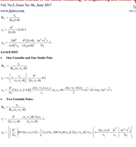
1 Yongho Lee et al. 2.0 1.7 4.1
2 Proposed (Improved) 0.29 1 4.32
Sr. No. Method
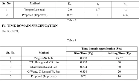
Time domain specification (Sec) Rise Time (TR) Settling Time (TS)
1 Ziegler-Nichols 0.833 45.67
2 C.T. Huang and Y.S. Lin 0.833 30
3 Shamsuzzoha and Lee 0.834 30
4 Q.Wang, C. Lu and W. Pan 0.836 20
440 | P a g e
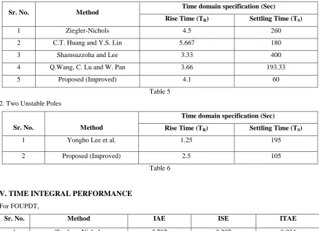
1. One Unstable and One Stable Pole
Sr. No. Method Time domain specification (Sec)
Rise Time (TR) Settling Time (TS)
1 Ziegler-Nichols 4.5 260
2 C.T. Huang and Y.S. Lin 5.667 180
3 Shamsuzzoha and Lee 3.33 400
4 Q.Wang, C. Lu and W. Pan 3.66 193.33
5 Proposed (Improved) 4.1 60
Table 5
2. Two Unstable Poles
Sr. No. Method
Time domain specification (Sec)
Rise Time (TR) Settling Time (TS)
1 Yongho Lee et al. 1.25 195
2 Proposed (Improved) 2.5 105
Table 6
V. TIME INTEGRAL PERFORMANCE
For FOUPDT,
Sr. No. Method IAE ISE ITAE
1 Ziegler – Nichols 3.702 3.287 9.054
2 C.T. Huang and Y.S. Lin 4.446 4.098 13.01
3 Shamsuzzoha and Lee 2.462 2.408 3.813
4 Q.Wang, C. Lu and W. Pan 3.07 3.064 5.664
5 Proposed (Improved) 4.32 3.246 14.37
Table 7
For SOUPDT,
1. One Unstable and One Stable Pole
Sr.No. Method IAE ISE ITAE
1 Ziegler – Nichols 43.47 38.15 1324
2 Tayrus-Luyben 49.79 62.91 1201
3 C.T. Huang and Y.S. Lin 37.03 22.38 1400
4 Poulin and Pomerleau 16.96 12.79 245.2
5 Proposed (Improved) 10.92 6.237 110.3
Table 8
441 | P a g e
Sr.No. Method IAE ISE ITAE
1 Yongho Lee et al. 7.729 2.489 131
2 Proposed (Improved) 6.369 2.87 56.31
Table 9
V. SIMULATION RESULTS
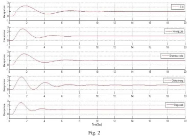
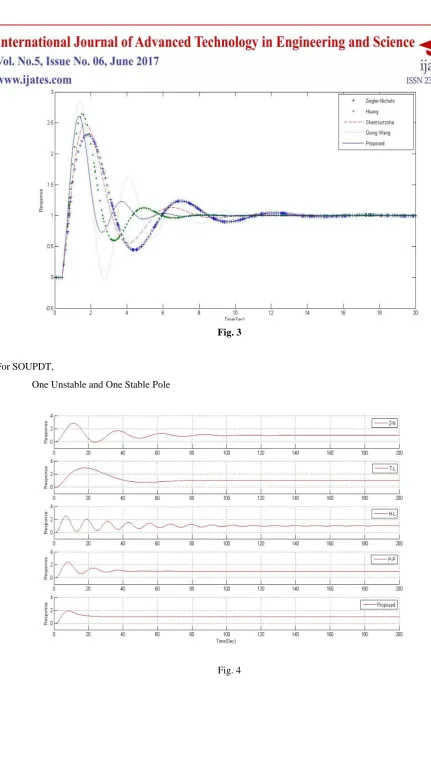
Fig. 2 and 3 shows PID controller performance by proposed and each considered method and comparison of these
methods for FOUPDT system.
Fig. 4 and 5 shows PID controller performance by proposed and each considered method and comparison of these
methods for SOUPDT (One Unstable and One Stable Pole) system.
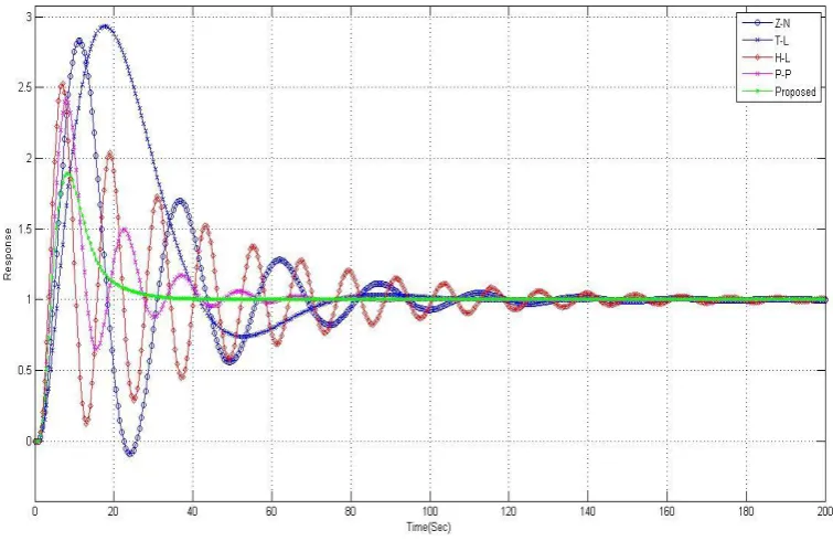
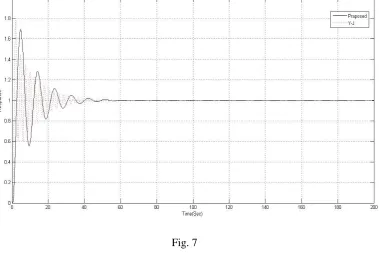
Fig. 6 and 7 shows PID controller performance by proposed and each considered method and comparison of these
methods for SOUPDT (Two Unstable Poles) system.
For FOUPDT,
442 | P a g e
Fig. 3
For SOUPDT,
One Unstable and One Stable Pole
443 | P a g e
Fig. 5
Two Unstable Poles
444 | P a g e
Fig. 7
VI. RESULTS AND DISCUSSION
Controller parameters calculated by tuning, these parameters make inverse effect to each other for optimum value of
controller. Proposed and other considered methods used for controller design for seeing which design method gives
good stability of the controller response. Time domain specification shows rise and settling time of controller,
minimum rise and settling time needed for good response of controller. Time integral performance shows different
error like IAE, ISE, and ITAE, which shows controller robustness.
VII. CONCLUSION
PID controller designed for FOUPDT and SOUPDT by Proposed and other considered controller tuning methods.
All methods are work in direction of settling the process variable to a desired set value. In FOUPDT, time domain
specification shows proposed method have less rise and settling time compared to other method and time integral
performance shows proposed method have IAE, ISE and ITAE are minimum compared to C.T. Huang and Y.S. Lin
method and maximum compared to other controller tuning methods for FOUPDT system. However, on time basis
proposed method is better response and shows good stability this shows that proposed method for first order
unstable process without taking too much time and oscillation for attain stability of the system. In SOUPDT, for one
unstable and one stable pole, Time domain specification shows proposed method have more rise time compared to
other method but less settling time. Controller stability and time integral performance shows proposed method have
IAE, ISE and ITAE are minimum compared to other controller tuning method this shows this method gives very
good stability and robust response of controller for second order unstable process without taking too much time and
oscillation for attain stability of the system. In case of two unstable poles, Time domain specification shows
proposed method have more rise time compared to other method but less settling time. Controller stability and time
integral performance shows proposed method have IAE, ISE and ITAE are minimum compared to other controller
tuning method this shows this method gives very good stability and robust response of controller for second order
445 | P a g e
REFERENCES
[1.] Shamsuzzoha, M.; Lee, M.IMC-PID controller design for improved disturbance rejection of time delayed
processes; Ind. Eng. Chen. Res.2007; 46, 2077-2091.
[2.] Huang, C. T., & Lin, Y. S. Tuning PID controller for open-loop unstable processes with time delay. Chemical
Engineering Communications, 1995;133, 11.
[3.] Poulin, ED., & Pomerleau, A.PID tuning for integrating and unstable processes. IEE Process Control Theory
and Application, 1996; 143(5), 429.
[4.] Qing Wang, Changhou Lu, Wei Pan, IMC PID controller tuning for stable and unstable processes with time
delay, Chemical Engineering Research and Design, 2015; 42.
[5.] Seborg, Edgar, Mellichap, Doyle Process Dynamics and control;2011; Edition 3rd page no. 223-225. [6.] Donald R. Coughanour,Process System Analysis and Control;1991;Edition 2ndpage no. 54
[7.] Yongho Lee, Jeongseok Lee, Sunwan Park, PID controller tuning for integrating and unstable processes with
time delay Chemical Engineering Science;1999; 55(2000) 3481-3483.
[8.] Desborough, L. D.; Miller, R. M. Increasing customer value of industrial control performance
monitoringHoneywell’s experience;Chemical Process Control −VI (Tuscon, Arizona, Jan. 2001). AIChE Symp. Ser. No. 326. 2002, 98.
[9.] Kano, M.; Ogawa, M. The state of art in chemical process control in Japan: Good practice and questionnaire
survey. J. Process Control 2010, 20, 969−982.
[10.]Tyreus, B. D.; Luyben, W. L. Tuning PI controllers for integrator/dead time processes. Ind. Eng. Chem. Res.
1992, 2625−2628.
[11.]Shahian, B., & Hassul, M. Control system design using MATLAB. Englewood Cli!s, 1993; NJ: Prentice Hall.
[12.]Padma Sree, R., Srinivasan, M. N., &Chidambaram, M., A simple method of tuning PID controllers for stable
and unstable FOPTD systems. Computers and Chemical Engineering, 2004, 2201–2218.
[13.]M. Ramasamy, S. Sundaramoorthy PID controller tuning for desired closed loop response for SISO system
using impulse response, Computers and Chemical Engineering, 2008, 1773–1788.
[14.]De Paor, A. M., Controllers of Ziegler-Nichols type for unstable process with time delay. International Journal
of Control, 1989, 1273.
[15.]Huang, H. P., & Chen, C. C., Control-system synthesis for open-loop unstable process with time delay. IEE
Process-Control theory and Application, 1997, 144.