University of Pennsylvania
ScholarlyCommons
Publicly Accessible Penn Dissertations
Summer 8-14-2009
Optimization of Multidimensional Nuclear
Magnetic Resonance Spectroscopy, for Resolution
and Sensitivity, Through Application of Radial
Sampling
John M. GledhillUniversity of Pennsylvania, [email protected]
Follow this and additional works at:http://repository.upenn.edu/edissertations Part of theOther Biochemistry, Biophysics, and Structural Biology Commons
This paper is posted at ScholarlyCommons.http://repository.upenn.edu/edissertations/19 For more information, please [email protected].
Recommended Citation
Gledhill, John M., "Optimization of Multidimensional Nuclear Magnetic Resonance Spectroscopy, for Resolution and Sensitivity, Through Application of Radial Sampling" (2009).Publicly Accessible Penn Dissertations. 19.
Optimization of Multidimensional Nuclear Magnetic Resonance
Spectroscopy, for Resolution and Sensitivity, Through Application of
Radial Sampling
Abstract
The high probability of degenerate frequencies in NMR spectra of complex biopolymers such as proteins presented a great barrier to detailed analysis. The combination of multidimensional NMR spectroscopy and high magnetic field strengths has overcome the resulting resonance assignment problem for proteins less than 50 kDa. However, as protein size increases the sampling and sensitivity limited regimes become apparent. As a consequence, the orthogonal linear sampling requirements of conventional multidimensional NMR
spectroscopy, combined with increased signal averaging require a longer acquisition time than is feasible. To overcome these limitations, radial sampling of the indirect dimensions of multidimensional experiments is utilized. It is demonstrated here, that through optimization of radial sampling acquisition parameters, it is possible to escape the linear sequential sampling requirements of Cartesian sampling, which allows for the collection of a high resolution spectrum in reduced acquisition time. Further, by exploiting a fundamental statistical advantage of radial sampling, it is possible to obtain a signal-to-noise advantage, over the traditional methodology. The approach is generalized by developing an all inclusive NMR data processing package and associated programs to optimize radial sampling acquisition parameters. An example, which utilizes the resolution and sensitivity advantages, to collect a novel application of a high resolution four-dimensional 13C, 15N edited NOESY is presented in support.
Degree Type
Dissertation
Degree Name
Doctor of Philosophy (PhD)
Graduate Group
Biochemistry & Molecular Biophysics
First Advisor
A. Joshua Wand
Keywords
NMR, Radial Sampling, Data Processing
Subject Categories
Other Biochemistry, Biophysics, and Structural Biology
COPYRIGHT
John Michael Gledhill, Jr.
iii Dedication
iv
Acknowledgements
Foremost, I would like to thank my wife, Charleen, for her loving support and
encouragement. She has truly played an unseen, but pivotal, role in all of this work. She
is amazing in the way she always knows exactly what to say to keep me going. But
realistically, most of the time, she doesn’t need to say anything because her smile says it
all.
I am also very grateful of my thesis advisor, Josh Wand, who has made all of this
work possible. His time, resources and capabilities have been essential. He has given me
the freedom to choose my path, but always been available to help define the details.
Thanks are also due to the members of the Wand Lab, both former and current,
especially, Kathy Valentine, Ron Peterson and Mike Marlow for helping me get started in
the lab and always putting up with my incessant questions. Jakob Dogan, has provided
great insight on pulse sequence development. Sabrina Bedard, Sarah Chung, Vignesh
Kasinath, Joe Kielec, Vonni Moorman, Nathaniel Nucci and Shoshanna Pokras have all
influenced this work.
Finally, I would like to thank my family and friends, all of whom, have played an
v ABSTRACT
Optimization of Multidimensional Nuclear Magnetic Resonance Spectroscopy, for
Resolution and Sensitivity, through Application of Radial Sampling
John M. Gledhill, Jr.
Dr. A. Joshua Wand
The high probability of degenerate frequencies in NMR spectra of complex
biopolymers such as proteins presented a great barrier to detailed analysis. The
combination of multidimensional NMR spectroscopy and high magnetic field strengths
has overcome the resulting resonance assignment problem for proteins less than 50 kDa.
However, as protein size increases the sampling and sensitivity limited regimes become
apparent. As a consequence, the orthogonal linear sampling requirements of conventional
multidimensional NMR spectroscopy, combined with increased signal averaging require
a longer acquisition time than is feasible. To overcome these limitations, radial sampling
of the indirect dimensions of multidimensional experiments is utilized. It is demonstrated
here, that through optimization of radial sampling acquisition parameters, it is possible to
escape the linear sequential sampling requirements of Cartesian sampling, which allows
for the collection of a high resolution spectrum in reduced acquisition time. Further, by
exploiting a fundamental statistical advantage of radial sampling, it is possible to obtain a
vi
by developing an all inclusive NMR data processing package and associated programs to
optimize radial sampling acquisition parameters. An example, which utilizes the
resolution and sensitivity advantages, to collect a novel application of a high resolution
vii
TABLE OF CONTENTS
CHAPTER 1. INTRODUCTION AND OBJECTIVES 1
CHAPTER 2. SPECTRAL ESTIMATION AND SPARSE SAMPLING 9
CHAPTER 3. AL NMR:AMULTIDIMENSIONAL NMRDATA PROCESSING
PACKAGE FOR CARTESIAN AND SPARSE SAMPLED DATA
34
CHAPTER 4. PHASING SPARSE SAMPLED MULTIDIMENSIONAL NMRDATA 64
CHAPTER 5. OPTIMIZED ANGLE SELECTION FOR RADIAL SAMPLED NMR
EXPERIMENTS
81
CHAPTER 6. SENDNMR:SENSITIVITY ENHANCED N-DIMENSIONAL NMR 112
CHAPTER 7. ANOVEL APPROACH TO RADIALLY SAMPLING THE 4D15N,
13C EDITED NOESY
131
viii LIST OF TABLES
TABLE 4.1 PROCEDURE FOR GENERATING ABSORPTIVE AND DISPERSIVE
SPECTRA
ix
LISTOFFIGURES
FIGURE 1.1 COMPARISON OF THE MOLECULAR WEIGHT OF PROTEIN
STRUCTURES DETERMINED BY NMR WITH THE MOLECULAR WEIGHT OF PROTEIN DRUG TARGETS
3
FIGURE 1.2 EXAMPLE OF INCREASING THE DIMENSION OF A NMR
EXPERIMENT TO INCREASE RESOLUTION
5
FIGURE 2.1 EXAMPLE OF SPECTRAL ESTIMATION 11
FIGURE 2.2 COMPARISON OF SAMPLING POINTS AND RESOLUTION 15
FIGURE 2.3 SAMPLING SCHEME COMPARISON 16
FIGURE 2.4 SCHEMATIC OF THE PROJECTION RECONSTRUCTION APPROACH 21
FIGURE 2.5 DEMONSTRATION OF THE LOWER VALUE COMPARISON 24
FIGURE 2.6 DEMONSTRATION OF THE FUNDAMENTAL LIMITATION OF
PROJECTION RECONSTRUCTION
26
FIGURE 2.7 EXAMPLE OF THE RESULTING SPECTRUM AFTER A SINGLE STEP
TWO-DIMENSIONAL FOURIER TRANSFORM
28
FIGURE 2.8 SPECTRUM SAMPLING SCHEME COMPARISON 29
FIGURE 2.9 SENSITIVITY COMPARISON OF THE VARIOUS SAMPLING
SCHEMES
x
FIGURE 3.1 RADIAL SAMPLING DATA PROCESSING EXAMPLE 36
FIGURE 3.2 AL NMR PROGRAM ARCHITECTURE 40
FIGURE 3.3 DEMONSTRATION OF THE INTRINSIC FLEXIBILITY OF THE
2D-FT
51
FIGURE 3.4 15NHSQC PROCESSING SCRIPT FLOW CHART 53
FIGURE 3.5 AL NMR INTERACTIVE PHASE CORRECTION INTERFACE 57
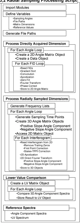
FIGURE 3.6 3D RADIAL SAMPLING SCRIPT FLOW CHART 60
FIGURE 4.1 EXAMPLE OF HOW QUADRATURE IMAGES ARE RESOLVED WITH
THE 2D-FT
68
FIGURE 4.2 THE 2D-FT CAN BE USED TO GENERATE ABSORPTIVE AND
DISPERSIVE SPECTRA
71
FIGURE 4.3 EXAMPLE OF THE PURE ±SAMPLING ANGLE REAL AND
IMAGINARY COMPONENT SPECTRA
73
FIGURE 4.4 COMPARISON OF PROCESSED SPECTRA WITH AND WITHOUT
PHASE CORRECTION
79
xi
FIGURE 5.2 ILLUSTRATION OF HOW RADIAL SAMPLING CAN SPEED
ACQUISITION
95
FIGURE 5.3 DEMONSTRATION OF ITERATIVE ANGLE SELECTION AND
SPECTRUM ANALYSIS
101
FIGURE 5.4 DEMONSTRATION OF THE MINIMUM ANGLES NEEDED TO
DETERMINE THE PEAK INTENSITIES
104
FIGURE 5.5 EXAMPLE OF CALCULATING THE FEWEST ANGLES NEEDED TO
GENERATE AN ARTIFACT FREE HNCO SPECTRUM
106
FIGURE 5.6 ITERATIVE ANGLE SELECTION TO GENERATE AN ARTIFACT
FREE HNCO SPECTRUM
108
FIGURE 6.1 RATIO OF MAXIMUM SIGNAL INTENSITY OF CARTESIAN
SAMPLING TO RADIAL SAMPLING
114
FIGURE 6.2 EFFECT OF THE LOWER MAGNITUDE COMPARISON ON
SPECTRUM NOISE
120
FIGURE 6.3 DENSITY ANALYSIS TO RETAIN A PEAK DURING LOWER VALUE
COMPARISON
121
FIGURE 6.4 MINIMUM SIGNAL-TO-NOISE TO RETAIN A PEAK 123
xii
FIGURE 6.6 COMPARISON OF SEND OPTIMIZED RADIAL SAMPLING AND
CARTESIAN SAMPLING
127
FIGURE 7.1 EXAMPLE OF THE DIFFICULTY OF USING THE INDIRECT PROTON
DIMENSIONS OF THE 3D15N FILTERED NOESY EXPERIMENT FOR ANGLE SELECTION
133
FIGURE 7.2 13C,15N EDITED NOESY PULSE SEQUENCE 135
FIGURE 7.3 EXAMPLE OF USING THE 4D RADIAL SAMPLED 13C,15N EDITED
NOESY PULSE SEQUENCE TO RESOLVE THE DEGENERACY
142
FIGURE 7.4 EXAMPLE OF EXTRACTING VECTORS FROM THE INDIVIDUAL
COMPONENT ANGLE PLANES
144
FIGURE 7.5 COMPARISON OF NORMALIZED PEAK INTENSITIES FROM THE
TRADITIONAL 3D AND NEW 4D NOESY PULSE SEQUENCES
1
CHAPTER 1
Introduction and Objectives
1.1 Introduction
In general terms, a protein's function is completely determined by its structure.
Understanding protein structure, in many cases, can elucidate functional understanding of
the protein at a mechanistic level. Stucture-function analysis has proven particularly
important in such topics as catalysis, ligand binding, molecular transport and signaling
cascades[1]. Protein structure has also played a pivotal role in understanding protein-drug
interaction and substantial effort has been applied to rational drug design[2, 3].
Crystallography and nuclear magnetic resonance (NMR) are the primary
techniques used to determine protein atomic structure. While crystallography has
outpaced NMR in the number of protein structure determined, the additional functionality
of NMR makes it appealing in many cases[4]. Namely, NMR allows for biophysical
characterization of proteins at site resolved resolution while the protein is in solution.
Though NMR has many appealing properties, until recently, the size range of proteins
amenable to analysis by NMR is not as broad as the size of proteins that are desirable to
study.
The disparity between proteins amenable to NMR analysis and those desired to be
studied arises from physical properties of the molecule and means by which NMR signal
2
accordingly the spin-spin relaxation rate, T2, decreases. An increase in T2 relaxation
results in broadened lineshapes and decreased scaler coupling transfer efficiency.
Unfortunately, these results decrease the signal to noise of the spectrum and limit the
application of some pulse sequences from the reduced coupling efficiency. Combined,
these effects have limited protein analysis beyond 35kDa.
Multiple methods have been developed in order to reduce the problematic effects
of slow molecular tumbling. The most effective have been extensive deuteration[5-7],
TROSY[8] pulse sequence optimization and reverse micelle technology[9]. Extensive
deuteration of the protein reduces the dipolar field surrounding the remaining protons and
in turn, eliminates many of the spin-spin relaxation modes. With application of deuterium
decoupling, this technique has allowed for application of multidimensional NMR
experiments to proteins in the 20kDa range[5-7]. TROSY (transverse relaxation
optimized spectroscopy) pulse sequences increase the functional protein size by selecting
for constructive interference between dipole-dipole relaxation, which arises from slow
molecular tumbling, and intrinsic chemical shift anisotropy. Cancellation of the
relaxation components allows for selection of a narrow lineshape component. This
technique has successfully been applied to proteins beyond 40kDa[10, 11]. The final
method to increase the amenable protein size range is application of reverse micelle
technology. Reverse micelles are created by encapsulating a protein, which is dissolved
in a small pool of water, inside a surfactant micelle that is dissolved in a non-polar, low
3
proteins is reduced. In turn, all traditional NMR methodology is applicable. This method
has been successfully applied to proteins great than 50 kDa[12](unpublished data).
Although the technology is available to study large proteins with NMR, the size
range, of protein structure determined by NMR, is not comparable to the size range of
proteins of interest. This disparity is apparent if the size of protein structures determined
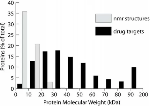
by NMR[13] is compared to the size of protein drug targets[14], Figure 1.1.
Figure 1.1 A comparison of the molecular weight of protein structures determined by NMR with the molecular weight of protein drug targets, is shown here. The relative frequency versus protein molecular weight demonstrates the disparity, in protein size, between proteins currently being studied and the size of proteins with desirable properties to study. NMR structure information was obtained from the PDB[13] and edited for redundancy. Drug target information was obtained from DrugBank[14].
The lag in protein structure size can be rationalized with the following two reasons: First,
the NMR methods available for large proteins function by decreasing the linewidth of the
4
do not account for the added complexity that arises from the increased the number of
signals in large proteins. Second, these methods often function at limited sensitivity
compared to traditional techniques.
Spectral complexity increases with increasing protein size. In general, NMR
spectra contain at least one peak per amino acid residue of the protein. Although in many
experiments, such as a NOESY, multiple peaks per residue are present. The dispersion of
chemical shifts does not increase coincidently with increasing protein size. Therefore, an
increase in the number of peaks directly increases the number of peaks per spectral
volume and results in decreased spectral resolution. Spectral complexity is decreased by
increasing the dimensionality of the spectrum. Additional dimensions are added by
correlating additional atoms in the magnetization transfer pathway. This serves to reduce
the degeneracy of the spectrum by increasing the spectral area while retaining a constant
number of peaks. This concept is illustrated in Figure 1.2. Here, the number of peaks
remains constant but the dimensionality of the spectrum increases. Ubiquitin is used to
show the effect of increasing the dimension of the experiment. When one dimension is
evolved, amide protons in this case, very few of the peaks are resolved. Evolving two
dimensions, Figure 1.2b, resolves a large fraction of the peaks but degeneracy is still
present in the spectrum. When three dimensions are evolved all of the degeneracy is
5
Figure 1.2 An example of increasing the dimension of a NMR experiment to increase the resolution of the experiment is shown here. Ubiquitin is used in all three panels. A one-dimensional amdie 1H spectrum , panel a, a two-dimensional 15N-HSQC[15], panel b and a three-dimensional HNCO[16] resolve an increasing number of peaks as the dimensionality increases.
Increasing the dimensionality of an experiment comes at the expense of
acquisition time. The total acquisition time of an experiment is estimated from the
product of the number of data points collected in each dimension, the number of transient
scans averaged per FID, the interscan, magnetization recovery, delay and the acquisition
time of each scan.
1
1 1
N
fid j s a
j
n − n n d t
=
=
∏
Here nj is the total number of points in dimension j of N total dimensions, ns is the
number of transients, and d1 and ta are the recyle delay and acquisition times respectively.
The length of the pulse sequence is comparatively small and ignored. Assuming minimal
6
acquisition time quickly increases beyond a reasonable range as the dimensionality of an
experiment is increased. Using the above parameters a 3D experiment would require .5
hour, a 4D 9 hours, 5D 12 days and a 6D 1.1 years[17]. Even using a minimal acquisition
scheme the total acquisition time expands beyond a feasible range beyond four
dimensions. Collectively this regime is known as the sampling limit[18]. In this regime
acceptable resolution determines the total acquisition time.
Sensitivity is the second limiting parameter to large protein structure
determination. Limiting sensitivity arises from dilute samples and/or complex sample
preparation protocols. In the case of large proteins, the problems are further compounded
by the technologies employed to circumvent tumbling limitations. Extensive, or factional,
deuteration decrease the dipolar field but limit the concentration of observable signal by
randomly exchanging the observable proton with a non-observed deuterium[6]. TROSY
techniques achieve a narrow peak by splitting the signal into four components and
selecting for one of the four components that has ideal relaxation parameters, in turn,
decreasing the observed signal by 75 percent[8]. Reverse micelles decrease the molecular
reorientation time by dissolving the protein in a low viscosity solvent. To minimize the
reorientation time, short chained hydrocarbons are used as a solvent. These solvents
require pressuring the sample in a special apparatus which limits the sample volume.
Some high-pressure NMR tubes limit volume by 67.5%[19]. Further, the concentration of
protein filled reverse micelles is limited by the amount of surfactant that can be added
7
Typically, when large protein techniques are used, sensitivity is increased by
averaging additional transients at the expense of additional measurement time. The
variance sum law dictates that doubling the number of transients averaged, which doubles
the acquisition time, will increase the signal to noise by the square root of 2. This regime
is known as the sensitivity limit[18]. Here the minimal acquisition time is determined by
the sensitivity of the experiment. Resolution is also typically limited in this regime
because time is spent collecting a large number of scans rather than an increasing number
of increments.
In light of the sampling and sensitivity limits, approaches are necessary to collect
data with increased resolution, without an exponential increase in acquisition time while
achieving a concomitant increase in sensitivity. Recently, various methods have been
introduced to speed acquisition. However, no new approaches are available to increase
the sensitivity of multidimensional NMR experiments.
All of the recent methods to speed acquisition rely on sparse sampling. In general,
sparse sampling speeds acquisition by reducing the number of data points collected in the
indirect dimensions. Typically, an order of magnitude time savings is possible using
sparse sampling.
1.2 Objectives
The primary objective of this thesis is to alleviate the resolution and sensitivity
8
The efforts are threefold: First the general application of sparse sampling is improved by
developing and extending current methodology. This includes a multidimensional NMR
processing program, designed to efficiently process sparse sampled data, chapter 3; novel
means to phase correct sparse sampled data, chapter 4; and an optimized sampling angle
selection routine for radial sampling, chapter 5. Second, means to obtain an increase in
sensitivity are developed. Termed, Sensitivity Enhanced n-Dimensional NMR (SEnD),
the approach is presented in chapter 6. Finally, focusing on the resolution and speed of
data acquisition, when radial sampling is employed, a new methods is developed. A novel
method to collect a 4D 13C, 15N edited NOESY spectrum is presented in chapter . The
results presented here are general and will facilitate development of additional novel
applications that exploit the acquisition speed, resolution and sensitivity advantages
9
CHAPTER 2
SPECTRAL ESTIMATION AND SPARSE SAMPLING
2.1 Introduction
In chapter 1 the sampling and sensitivity limited regimes[21] were presented. In
order to overcome these limits, new methods that increase the resolution and sensitivity
without a concomitant increase in acquisition time are needed. Of late, substantial work
has been performed to alleviate the sampling limits imposed by the strict linear sequential
sampling requirements of the standard fast Fourier transform. The majority of the new
techniques are base on sparse sampling. Sparse sampling decreases acquisition time by
selectively skipping acquisition of points in the indirect dimension. A substantial time
savings can be achieved by skipping acquisition points, but this comes at the expense of
spectral artifacts. Various spectral estimation methods have been developed to account
for or eliminate these artifacts. The various sampling schemes and processing techniques
will be reviewed here to determine which is most suitable for our applications.
Prior to reviewing the sparse sampling and data process techniques a review of
spectral estimation is presented. This review will serve to further clarify the fundamental
10
2.2 Spectral Estimation Review
NMR signal arises from the evolution of transverse magnetization[4]. As the
magnetization evolves a time-varying current is generated. This current is measured as a
time series of exponentially decaying sinusoid by the spectrometer. The time series data
can be represented as:
0, , ,1 M 1
d d d −
=
d … (2.1)
Where M is the total number of points sampled. In most cases a uniform increment is
used between data points to make the data amenable to processing techniques that will be
presented below. In all but the simplest cases, determining the underlying frequency
components is impossible from direct inspection. Therefore, the time data is converted to
the frequency domain using one of the various spectral estimation techniques. Estimation
of the frequency domain data from the time domain is represented as:
↔
d f (2.2)
Converting the data to the frequency domain allows for a measure of the frequency
components to be read directly from the resulting spectrum. The frequency series can be
represented as:
0, , ,1 N 1
f f f −
=
11
Where N is the total number of frequency components determined from the data. An
example of converting the time series data to the frequency domain is shown in Figure
2.1.
Figure 2.1 An example of spectral estimation is shown for generated data containing two peaks of varying intensity. The time series of an exponentially decaying sinusoid is shown on the left. Only the cosine modulated component is shown for clarity. Application of the Fourier transform to estimate the frequency spectrum produces the spectrum shown on the right.
Here an exponentially decaying sinusoid, of generated data containing two frequency
components of different amplitudes is shown. The frequency components are not easily
determined from visual inspection of the time data. Estimation of a frequency spectrum
allows for direct inspection of the frequency components. Additionally, the frequency
spectrum, allows for the relative intensity of the frequency components to be directly
assessed. This feature is particularly important when there is a large noise component in
12
The Fourier transform (FT)[22] is the most common method for spectral
estimation. The FT is appealing because it is a linear transform, which allows for the data
quality to be directly assessed from the noise level of the spectrum. It is also fast and has
no adjustable parameters, making application easy.
Efficient application of the FT requires that the data is sampled at a constant
interval. Utilizing a constant interval the data series is written formally as a summation of
sinusoids encompassing all of the detectable frequencies multiplied by an exponential
decay parameter, T2k.
2
1
/
0
cos(2 ) k
N
m T
k k
k
A πω m τ e τ
−
Δ
=
=
∑
Δd (2.4)
Where N is the total number of frequency components that can be determined, Ak is the
amplitude term of a given component k, with frequency ωk. m is the series point of M
total points and Δτ is the sampling increment. The sampling increment determines the
detectable frequency range as dictated by the Nyquist theorem[23]; which states that the
range of detectable frequency is ½ the inverse of the time increment. Therefore, if the
data is centered at zero frequency the detectable band of frequencies is: sw 1 τ
=
Δ . In
order to determine if a frequency component is positive or negative with respect to the
carrier quadrature detection is employed. Quadrature detection is accomplished by
13
and imaginary pair is stored as a series of complex numbers. Using the Eulers identity
and assuming the summation, the data series is written as:
1 1/ 2
i n n T
Ae−ω τΔ + Δτ =
d (2.5)
Having defined the possible frequency range of the data series, it is possible to
determine all frequencies are present in a given spectrum. The FT solves for the
amplitude of each frequency component by first generating a model sinusoid at the given
frequency using the same time points as the data. Then the amplitude is determined by
summing the product of the data and the sinusoid. The FT of the frequency series is
written as: 1 2 / 0 1 M kn M k k e M π − = =
∑
nf d (2.6)
The various terms have the same meaning as above. This representation utilizes the fact
that the time and frequency components do not need to be explicitly defined. If the
Nyquist sampling theorem is applied then the frequency and time points are both a
function of the sweep width and the two terms are reduced to nk
M . This generalization
assumes that the same number of frequency terms are determined as there are number of
data points and the points are equally distributed in the sweep width range. If 16 points
are collected, show in black, then the spectrum with broad lines is generated, black as
well. If an additional 48 points are collected, resulting in 64 total points then the resulting
14
expanded to multiple dimensions the limitations of Cartesian sampling are immediately
apparent.
When a multiple dimension experiment is collected, each dimension is sampled
independently and sequentially using a Cartesian basis. The resulting data is a product of
all of the time domains that are evolved.
1 1/ 2 2 2/ 2
i n n T i n n T
Ae−ω τΔ + Δτ e−ω τΔ + Δτ
=
d (2.7)
Sampling each dimension independently allows each dimension to be processed
independently. For example, in the case of a 2D experiment the data is collected with
respect to two incremented timesd t t( , )1 2 . This data is first Fourier transformed with
respect to t2, resulting in a mixed time-frequency spectrumd t f( ) ( )1 ω2 . The matrix is
then Fourier transformed with respect to t1, resulting in the frequency domain spectrum
1 2
( , )
f ω ω . The independence of each dimension requires that a sufficient number of data
points be collected to achieve suitable resolution, as discussed above. In turn, increasing
the dimensionality of the experiment exponentially increases the required acquisition
time.
Collecting a larger number of data points increases the digital resolution of the
frequency spectrum. As a secondary effect, the linewidth of peaks in the frequency
spectrum are also decreased. Typically, the time data is apodized prior to FT.
Apodization is the process of multiplying the data series by a decaying time function to
15
truncation artifacts and provides a more satisfactory line shape. When more data points
are present the apodization function brings the data to zero slower, which, when Fourier
transformed, results in a narrowed line. This concept is illustrated in Figure 2.2. To
circumvent an exponential increase in acquisition time alternate sampling and processing
schemes have been presented.
Figure 2.2 Increasing the number of time domain points acquired (left) directly increases the resolution of the frequency domain spectrum (right). The linewidth in the frequency spectrum is substantial decreased by increasing the number of points from 16 to 48.
2.3 Sparse Sampling
Sparse sampling decreases the acquisition time of multidimensional NMR
experiments, by reducing the number of points collected in the indirect dimensions. The
design of the spectrometer allows for the directly acquired dimension to be collected in
real time so only points in the indirect dimensions are sparsely sampled. Various sparse
16
suitable level of information while not reducing the spectral resolution. As a result of
incompletely sampling each dimension, the sparsely sampled dimensions contain
artifacts. The artifacts are directly dependent on the sampling scheme used, as well as the
method used to process the spectrum. A review of the various sample schemes and the
resulting artifacts are presented here. The sampling schemes are presented first, followed
by a discussion of the processing methods.
17
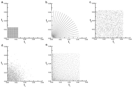
in d and optimized random sampling is shown in e. In all schemes a 2000 Hz sweep width was used in both dimensions.
A collection of the various sampling methods are shown in Figure 2.3. The plots
only show the sampling pattern for the indirect dimensions of a 3D experiment. As
above, the directly acquired dimension is sampled traditionally. All plots in the Figure
use the same number of sampling points, 50x50 over the two indirect dimensions.
However, all of the sparse sampling schemes are collected over the time domain space
equivalent to 128x128. This corresponds to a 6-fold time advantage for sparse sampling.
The sampling schemes can be divided into two main categories, radial sampling and
random sampling. Radial sampling, Figure 2.3b, is achieved by linking two or more of
the indirect dimensions and linearly sampling a vector at an angle (α) with respect to the
two orthogonal time domains. In the case of a three dimensional experiment, this is
achieved by collecting the directly detected time domain signal normally and linking the
indirect dimensions by defining t1 =τcos(α) and t2 =τsin(α) and linearly sampling the
time period τ[25]. In this case, only one time vector is sampled per two time dimensions.
Multiple angles are collected to resolve the degeneracy of collecting data in a lower
dimensional space.
Random sampling is the second class of sparse sampling schemes[26]. This
method is achieved by using a pseudo-random number generator to choose the
acquisition time points in the indirect dimensions. Typically the maximum evolution of
18
given time domain dimension. The first application of random sampling used a uniform
distribution of sampled points in the indirect time domains[26, 27], Figure 2.3c. Initial
applications of uniform random sampling demonstrated that a significant resolution
advantage can be achieved with this sampling protocol because only a gentle apodization
function is required to remove truncation artifacts. Additionally, in many cases the data
points are sampled at increments less than the Nyquist frequency which allows for more
accurate detection of chemical shifts. Although a higher resolution spectrum was realized
with uniform radial sampling artifacts were immediately apparent in the spectrum.
Details regarding the artifacts are discussed below. To reduce the detrimental effects of
the artifacts more sophisticated schemes have been proposed. These include Gaussian
weighted random sampling[28], Figure 2.3d. Here, a probability bias is applied to the
pseudo-random number generator. Weighting the distribution of sampled points reduces
the effects of the artifacts. Optimally, a Gaussian distribution would be used that matches
the decay properties of the nuclei evolved in the indirect dimensions.
Random sampling is further optimized by distributing the data points closer to a
Cartesian basis, while still retaining a level of random sampling. Optimized random
sampling[29], Figure 2.3e approaches a Cartesian approximation by placing additional
restraints on the time points sampled. When Optimized random sampling is used, a grid is
generated over the two indirect evolution time dimensions. The area of each cell in the
grid increases with a Gaussian weight as the evolution times increase. This sampling
19
still sampling enough points to avoid truncation artifacts. One data point is selected per
grid cell. Again this sampling method improved artifacts.
Further normalization of the sampling pattern led to the creation of concentric
shell sampling[30]. This sampling scheme produces an artifact free spectrum if specific
criteria are met. The sampling scheme functions by collecting data points that are equally
spaced on rings with expanding radii. The spacing of the points and rings are dependent
on the required sweep width of interest. This sampling scheme requires an equivalent
number of points as Cartesian sampling and therefore is not analyzed further here.
However, the number of sampling points can be reduced systematically to produce a
randomized scheme that is comparable to the optimized random sampling approach.
Regardless of the sampling scheme utilized, quadrature detection is still required
to determine the sign of a peak relative to the carrier frequency. This is achieved by
acquiring both a real, or cosine modulated component, and an imaginary, or sine
modulated component, per dimension. In the case of a 3D experiment, four quadrature
components are collected for the two indirect dimensions at each sampling time
point[25]. The four data components, represent all combinations of the even and odd
functions, which are Cos-Cos modulated, Cos-Sin, Sin-Cos and Sin-Sin. All four of the
components are used in the processing techniques that will be discussed.
Traditional sequential 1D Fourier transform data processing methods are no
20
two main classes of processing technology to deal with sparse sampled data: projection
reconstruction[25] and numerical estimation based[16, 17, 31-36]. The objectives of the
projection reconstruction techniques are to generate a final spectrum directly from the
data. Numerical estimation based techniques are generally designed to generate a list of
the spectral features, then either use the information to create a peak list or generate a
final spectrum. Projection reconstruction based techniques are only amenable to radial
sampling, while numerical estimation methods are amenable to both radial and random
sampling.
2.4 Projection Reconstruction
Application of projection reconstruction to NMR originated as an extension of
computerized tomography techniques[37]. In computerized tomography techniques,
multiple 2D ‘tilted plane’ projections of a 3-dimensional object are recorded as a function
of sampling angle. The 2D projections are then used, through application of the Radon
transform[38], to regenerate a representation of the 3D object. In the case of NMR
experiments, radial sampling is used to collect tilted planes of time domain data, which is
Fourier transformed to generated tilted planes in the frequency domain. However, unlike
tomography, NMR spectra contain discrete peaks rather than continuous objects. Discrete
peaks require fewer angles planes to regenerate a final spectrum. An example of the
21
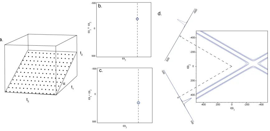
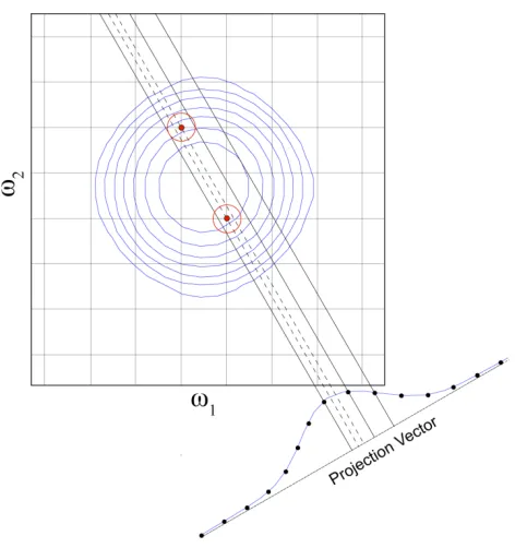
Figure 2.4 Schematic of the projection reconstruction approach to NMR. Radial sampling is use to sample a spectrum, a. To accomplish this, the directly acquired dimension, t3, is sampled using a Cartesian pattern.
The two indirect dimensions, t1 and t2, are linked and sampled simultaneously at an angle α (see text for
details). The directly detected dimension is processed with standard Fourier transform technology. The indirect dimension cannot be processed directly. From the four quadrature components, sum and differences, employing double angle identities, of the various components are used to generate two complex pairs. The two complex pairs are Fourier transformed, generating two spectrum with the signals modulated by the sum and difference of the frequency components. These spectra are the tilted planes. The sum and differences are shown in panels b and c, respectively. Each indirect vector of the two spectra are projected into the frequency components at 90± α. The two dashed lines in b and c indicate the example vectors used for reconstruction in d. Here, additive back projection is used to resolves the degeneracy of the individual spectra. The vectors are aligned from the carrier frequencies and projected along the
perpendicular into the two frequency domains. The intensity from each point on the tilted plane vector is added to the existing intensity in the frequency domains. This generates a ridge of intensity perpendicular to peaks. The peak chemical shift is located at the intersection of the ridge components.
Here, the directly acquired dimension is collected using Cartesian sampling while the two
22
directly detected dimension is processed using standard Fourier transform methodology.
This results in a 2D mixed mode spectrum, where d1 is frequency and d2 is an
interferogram of time domain data (not shown). The 2D plane is tilted between the two
indirect time dimensions. There are no means to distinguish a positive sampling angle
from a negative sampling angle. Therefore, double angle identity linear combinations of
the quadrature component spectra are calculated to separate the sum and difference of the
two frequency domain components[39]. The positive and negative frequency component
spectra are then used as a Fourier transform quadrature pair to generate the positive tilt
angle spectra, Figure 2.4b, and the other two used to generate the negative tilt angle
spectra, Figure 2.4c.
Information is not available to determine the peak location orthogonal to the tilted
spectrum plane. Two methods are commonly used to resolve the degeneracy: additive
back-projection and lower magnitude comparison[25]. Additive back-projection (ABP),
the equivalent of the radon transform, sums all of the component spectra with the
intensity, from the tilted plane spectrum projected along a vector orthogonal to the point
in the tilted plane[40]. This method produces a ridge of intensity wherever there are
peaks in the tilted plane spectrum, Figure 2.4d. When both the sum and difference
components are projected into the same spectrum, the ridge intensity constructively sums
at the location of ridge intersections. When there is only one peak, in the indirect plane,
the intersection of the two ridges corresponds to the chemical shift of the peak. When
23
chemical shifts, as well as an artifact peak location. Ridges always intersect at the
chemical shift of a peak, independent of the sampling angle. Multiple sampling angles are
added into the spectrum to determine authentic peaks from artifact peaks. Adding more
sampling angles to a spectrum will always reinforce peak intensity, while the artifact
peak will remain at a baseline level. This method is capable of producing a readable
spectrum, but suffers from severe baseline artifacts. The baseline artifacts can be
removed using lower value (LV) method[25]. This method generates a back-projected
spectrum for each of the component angles. The individual angle components are
compared on an element basis retaining the minimum magnitude intensity value at each
point. This removes all of the ridge intensity other than that from the authentic peaks,
because only the peaks will have a non-baseline value as the sampling angle is varied. An
24
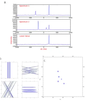
Figure 2.5 Demonstration of the lower value comparison. Panel shows a lower value comparison in 1D. The two spectra, 1 and 2, are compared point-to-point, and the smallest magnitude value is retained and stored in a third spectrum, labeled lower value. Note by comparison artifact peaks are removed. A 2D example, using a 3D radial sampled HNCO of Ubiquitin, is shown in b and c. (b) Four angle spectra are generated using ABP for each sampling angle; 0, 30, 45 and 90. (c) All four of the angle spectra are compared using the lower value to generate a final spectrum, which resolves all of the peaks.
The LV method efficiently removes artifacts from the spectrum, but has the potential to
remove authentic peaks from the spectra if the intensity of a peak falls into the noise for a
25
Two additional methods are also available to reconstruct a spectrum from the
component angle spectra: hybrid reconstruction[41] and distribution reconstruction[42].
Both of these methods were developed to avoid some of the pitfalls of ABP and LV.
When the S/N of the component spectra is limiting, peaks can potential be removed
during LV comparison. Hybrid reconstruction uses a combination of ABP and LV.
Starting with a set of component spectra sampled at various angles, the hybrid method
generates ABP spectra from a subset of the component spectra. The sub-group ABP
spectra are then used as input for a LV comparison to generate a final spectrum.
Generating sub-group ABP spectra prior to LV, the peak intensity is increased prior to
the LV, which decreases the likelihood that a peak will be inadvertently removed. The
distribution method functions by creating a histogram of intensity values from each of the
component spectra at the equivalent positions. A Gaussian is fit to the histogram and the
intensity value at the max value of the Gaussian is selected for the final spectrum. This
method proposes to avoid some of the flaws that are inherent to the other methods, but it
is much more computationally intensive.
Projection reconstruction techniques are digitally limited when projecting the
tilted planes into the final spectrum. Often, the data points of the tilted plane do not align
with the data points in the final spectrum. Points on the tilted plane must be interpolated
in order to determine the intensity values at the points in the final spectrum. This problem
26
Figure 2.6 Demonstration of the fundamental limitation of projection reconstruction. To demonstrate the problem, the projected vectors are overlaid on a Cartesian sampled spectrum to indicate the chemical shift. To generate a frequency spectrum, data points from the projection vector are extended into the frequency plane. Often the points of the tilted projection vector and the frequency plane do not coincide, because both the projection vector and frequency plane are discretely sampled. The red circles indicate two points that do not fall on the projected intensity. To determine the intensity value at these points, the intensity at the intersection of the dashed line and the projection vector need to be interpolated. The interpolation process is inaccurate and time consuming.
Two studies, APSY[43] and HIFI[44], have proposed to avoid reconstruction by only
using the peaks of a tilted plane spectrum. Under appropriate conditions these methods
have been successfully applied. However, by not generating a final spectrum all of the
existing analysis methodology is dismissed. Therefore, new means to directly solve for
27
tilted plane, have been presented to circumvent this limitation. This method realized that
the summation used in ABP is essentially a direct multidimensional Fourier transform[26,
45, 46].
2.5 Direct Two-Dimensional Fourier Transform
The direct multidimensional Fourier transform (2D-FT) functions by
simultaneously transforming multiple indirect dimensions as opposed to transforming the
dimensions sequentially. The discrete 2D –FT can be described as [45-47]:
1max 2max
1 2 1 1 2 2 1 2 1 2 1 2
1 0 2 0
( , ) exp( ) exp( ) ( , ) ( , ) ( , )
t t
t t
S ω ω i tω j t f t t g t t w t tω
= =
=
∑ ∑
− − (2.8)Where i and j are quarternion numbers; t1, t2 are the incremented times, ω1 and ω 2
comprise the frequency pair being determined, f t t( , ) exp(1 2 = − Ωi t1 1)exp(− Ωj t2 2) is the
data being transformed, Ω1 and Ω2 are the chemical shifts for time domain t1 and t2
respectively, w(t1,t2) is a weighting factor to account for the unequally spaced sampling
of the time domain and is typically applied as a two dimensional apodization function,
and g t t( , )1 2 describes the lifetime of the signal, which we will subsequently ignore. In
the case of radial sampling t1=τcosα andt2 =τsinα where τ is the incremented time
and α is the sampling angles.
An example of using the direct 2D-FT on generated data is shown in Figure 2.7.
28
to 45 degrees. The linewidth was adjusted to 10 Hz by multiplying the data sets by an
exponential decay. Further details using this same example are revisited in chapter 4.
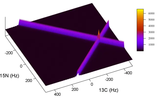
Figure 2.7 An example of the resulting spectrum after a single step two-dimensional Fourier transform. The data was generated with spectral parameters similar to that found in a radial sampled HNCO experiment. The sweep widths were set to 2000 and 1500 Hz for the t1 (carbon) and t2 (nitrogen) dimensions
respectively. One peak was simulated at -300, 75 hertz with a linewidth of 10 Hz. Radial sampling was
realized by incrementing the time in the first dimension as t1=(n sw1)cosα and the second dimension
as t2 =(n sw2)sinα.
Here, all of the points in the frequency domain were solved for rather than projected from
tilted planes. This avoids problems associated with interpolation of data points. However,
similar to the projection reconstruction approach, ridges still extend from the peak
chemical shifts. All of the methods to remove the ridges presented for projection
29
2.6 Comparison of Sparse Sampling Schemes
The direct multidimensional FT has an additional advantage over projection
reconstruction, namely it is amenable to any sampling scheme, not just radial sampling.
This occurs because the time points are explicitly defined in the 2D-FT, whereas, the PR
techniques use the FFT which assumes equally spaced time points. This allows for a
direct comparison of the various sampling schemes. Figure 2.8. shows the resulting
spectrum when the various sampling schemes are applied to a generated data set.
30
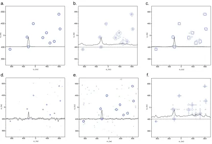
The uniform random, Gauss weighted random and optimized random samped spectra are shown in d., e. and f., respectively. All spectra were generated from 2500 points using the sampling time points shown in Figure 2.3. The data points for each spectrum were generated using Equation 2.7 using a summation of the ten frequency components seen in panel a. A 0.02 second T2 was used when generating the data for both
dimensions. All spectra were processed using a 2D-FT after applying apodization with a cosine squared function to remove truncation artifacts.
The Cartesian sampled spectrum is shown in Figure 2.8a for comparison. In all of the
experiments, the equivalent number of points were generated in order to keep the
potential signal volume constant. No noise was added to the generated data, this allows
for any baseline artifacts to be directly visible. A 1D slice is shown in all of the spectrum
to reference the baseline artifacts. Inspection of the spectrum for all of the sampling
schemes demonstrates that all of the peaks are accurately represented, while the baseline
artifacts vary for each method. All of the random sampling schemes produce baseline
artifacts that appear as noise. Randomized concentric ring sampling also produces
baseline artifacts (results not shown). Radial sampling also has baseline artifacts from the
ridges extending from all of the peaks, as a function of sampling angle, when no ridge
removal technique is applied. When LV comparison is applied the baseline artifacts are
removed. To determine the effect of baseline artifacts on the spectrum the signal to noise
for the various sampling methods spectra are plotted as a function of data points sampled,
Figure 2.9. This figure illustrates the advantage of radial sampling over all of the other
31
Figure 2.9 Sensitivity Comparison of the various sampling schemes as a function of number of points acquired. The S/N of each spectrum shown in Figure 2.8 is analyzed here. Each point is the average S/N of all 10 peaks in the spectra averaged. When Cartesian sampling was measured the number of points was always increased equally in both dimensions, retaining a square grid. When analyzing radial sampling the number of angles was increased, using approximately 100 points per angle. For the other sampling schemes the points were distributed according to the probability distribution of each sampling type.
2.7 Numerical Methods of Spectral Estimation
Numerical methods are also available to perform the spectra estimation of a
frequency domain spectrum on sparse sampled data[16, 17, 31-36]. The general objective
of numerical methods is to solve for the spectral parameters, such as the peak chemical
shifts, then use the information to generate a final spectrum. In many cases, it is very
difficult to generate an accurate representation of the spectrum because the data is
32
generated spectrum is not a transform and therefore nonlinear, so the reliability of the
chemical shifts is no longer assessable from the noise level in the final spectrum. With
this said, methods based on a least-squares fit of estimation parameters to the data have
had limited success when the noise level increases; although multiple applications have
proven useful when the noise of the spectrum is limited. The successful applications
include filter diagonalization[16, 33], maximum likelihood[25, 31], MDD[34] and
GFT[17]. One additional method, Maximum Entropy[24], attempts to account for the
problems associated with least squares fit, and has had slightly broader success.
Although many successful applications of the various numerical methods have
been presented, the application of each technique is dependent upon the data quality and
the type of experiment being collected. In order for the work here to be generally
applicable the direct multidimensional FT is used here. In most cases numerical methods
can also be substituted when applicable.
2.8 Conclusion
Traditional Fourier transform technology requires a large number of data points to
achieve a high resolution spectrum. When multiple dimensions are required to resolve
spectral degeneracy, the time required to satisfy the linear sampling requirement
increases beyond the stability of the spectrometer. Application of sparse sampling allows
circumvention of the time limitation of high dimensional NMR experiments. The 2D-FT
33
collected with any sampling scheme and its ability to directly access the data quality
through the noise level of the spectrum.
Comparison of the sampling schemes spectra demonstrate that radial sampling is
preferred because of the predictability and ease of removal of the artifacts. Also, the
smooth baseline outside of the artifact ridges have superior spectral characteristics
compared to the artifacts from random sampling that appear as baseline noise. Finally,
comparing the S/N of processed spectra from the various sampling schemes demonstrate
that there is a possible sensitivity advantage when using radial sampling combined with
34
Chapter 3
Al NMR: A Multidimensional NMR Data Processing Package for Cartesian and Arbitrarily Sampled Data
3.1 Introduction
From the previous chapters it should be apparent that the time and resolution
advantages of sparse sampling make its general application very appealing. This is
especially true in the case of large proteins. As protein molecular weight increases, quite
often spectral degeneracy increases concomitantly. Sparse sampling offers an increase in
acquisition time which enables higher dimensional experiments to be collected in the
same time as the lower dimensional analog.
Although methodology has been developed that utilizes the gains of sparse
sampling processed with a direct multidimensional Fourier transform (2D-FT)[27,
48-50]. There is no program available generally available to handle all aspects of sparse
sampled data processing. Typically a combination of current processing programs and an
external 'in-house' program is utilized for processing. Subsequently, convential programs
are available to display and analyze the data, such as, Sparky[51] or Felix (Felix NMR,
35
Two programs are used to process the data because the directly detected
dimension is processed with traditional fast Fourier transform methodology, while the
indirect dimensions, that utilized a sparse sampling pattern, are processed with a direct
multidimensional Fourier transform. In order to process all aspect of sparsely sampled
data, including the direct and indirect dimensions, a new data processing package is
presented here.
Al NMR incorporates all traditional NMR data processing methodology and new
multidimensional Fourier transformed based methodology. The processing program is
based on the python scripting language which is becoming one of the standard languages
in scientific data analysis. Further, multiple programs, XPLOR-NIH[52] and Sparky[51],
familiar to most NMR spectroscopists, utilized the python language.
3.2 Sparse sampling data processing with direct 2D-FT
To demonstrate the processing procedure, a simple example, employing radial
sampling[25] for generated (3,2) data set is presented. Here radial sampling is
accomplished, in the case of a 3d experiment, by simultaneously evolving both
dimensions while collected the directly detected dimension normally. The simultaneously
evolved dimensions are set such that the incremented times are t1=τcos(a) and t2=τsin(a).
Where t is a common, linearly incremented time and a is the radial angle between the two
orthogonal time domains. An example of the time points sampled by radial sampling, for
36
angle between the two indirect dimensions. For each sampling point in the time domain
in Figure 3.1 there are 8 corresponding quadrature components, a real and imaginary for
each dimension.
Figure 3.1 Radial sampling data processing example for a 3D spectrum of generated data, with a single peak. a. The time points are collected using a Cartesian basis with respect to the directly acquired
dimension. Radial sampling is used in the indirect dimensions by sampling t1=τcos(a) and t2=τsin(a). A 45°
sampling angle is used. b. The directly acquired dimension is processed using a FFT which results in a mixed mode, frequency, ω3, time, tα spectrum. c. The direct 2D-FT is used to process the two indirect
dimensions which generates the final frequency domain spectrum.
To process the data set, the directly detected dimension, t3, which was collected
traditionally, is processed using traditional Fourier transform methodology[22]. Each
vector along, t3, is processed separately, as is typically done, including convolution,
apodization, zerofilling and Fourier transformation. Processing of t3 produces a mixed
mode spectrum, Figure 3.1b. The spectrum is in the frequency domain along w3 and the
indirect dimensions are still in the time domain. The intensity of the peaks along w3 is
37
produces an interferogram along the radial sampling angle. For clarity, only one of the
four quadrature components is shown in the Figure.
After the directly detected dimension is processed, the two indirect dimensions
are processed simultaneously using the direct 2D-FT[45-47]. The 2D-FT generates a 2D
frequency matrix for each vector perpendicular to w3. Typically, each vector is apodized,
using a 2D apodization function, or weighed[27] before processing with the direct
2D-FT. The resulting 3D spectrum, after all processing, is shown in Figure 3.1c. As a result
of the indirect time domains being underdetermined artifact ridges extend from the
authentic peak chemical shifts at 90 +/- the sampling angle. The artifact removal methods
for projection reconstruction can be applied here to generate a final, artifact free,
spectrum.
The direct 2D-FT is discrete, which requires, that all of the time points and
frequency pair values are supplied to the function. By supplying all of the necessary
parameters allows the 2D-FT to process data regardless of the sampling scheme
employed.
Randomly sampled data is processed using the same flow of operations as
presented for radialy sampled data. The random sampled data is collected traditionally in
the directly detected dimension and processed with the FFT. The indirect dimensions are
sampled simultaneously by randomly selecting coordinate times in the evolution domains
38
2D-FT to generate a final frequency domain spectrum. Prior to application of the direct
2D-FT the data can be weighted or apodized to increase the resulting spectrum quality.
The random time point selections can be modified by weighting the selection criteria to
reduce artifacts that are intrinsic to the sampling scheme.
3.3 Al NMR Program Architecture
Al NMR is designed to be a standalone processing package. It does not depend on
any of the currently available processing packages for functionality. By designing the
program in a self contained manner, allows for increased flexibility to process data
collected with arbitrary sampling schemes and dimensions. Additionally, the program is
designed to be extendable, by the end user, to develop new methodology. To achieve this
flexibility Al NMR uses a Python interface[53]. Python is an established, efficient
scripting language. The language is easily learned. Currently, multiple programs,
designed for NMR utilize a Python interface. By designing the program as a standalone
module data processing is streamlined. Raw data is read directly from the spectrometer
and a processed output spectrum is generated. Utilizing Python no scripts needs to be
compiled.
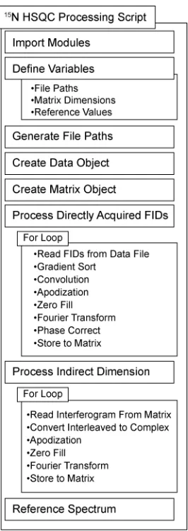
The program architecture is shown in Figure 3.2. All aspects of the program are
controlled by the user, either through the command line or by a user supplied script. The
39
functionality of the program. Typically a script will, at a minimum, load the Al NMR
module, read the data from the spectrometer file, process the time domain data into the
frequency domain and generate a processed matrix file. All of these commands, listed in
the script, are parsed by the python interrupter and passed to the python engine. The first
step when a script is executed is to load the Al NMR module. The module extends
pythons functionality to include reading, writing and processing NMR data. All of the
standard python functionality is retained. With direction from the script, the program
reads the NMR data file and creates a data object. The data object includes all of the
relevant acquisition parameters and access to the FIDs. Currently, the program supports
either Varian or Bruker data files. Further direction of the script controls access of FIDs
from the data object and process of the FIDs. In many cases each FID is processed
identically. This step can be performed in a parallel using built-in python functions.
Finally, the script controls creation of a matrix file object which interfaces with a final
40
Figure 3.2 Al NMR program architecture.
Python makes up the core of the processing program. Python is one of the most
popular, cross platform scripting languages available. Because it is a scripting language
the end user doesn’t need compile scripts and scripts are easily shared with a colleague
using a different operating system. Further, because of the popularity of python there is a
large body of tutorial and books available to learn the language. Additionally, when
debugging a script the large support environment is advantageous as compared to a
41
Technically, python is desirable because it takes care of all of the overhead in
developing a scripting package. It includes means for command interpretation on the
command line and through scripts. All methods of looping and computational details
such as memory allocation are available. Additionally, utilizing python, scripts can
developed easily that include technically complicated concepts such as queuing and
multithreading. Finally, utilizing python the core functionality can be expanded with a
library of user developed codes. This allows for the package to be extended to meet any
users needs.
3.4 Python introduction
An introduction to the python scripting language is presented here to assist the
user with developing scripts. Only salient features of the scripting language are presented.
The user is referred to many good online tutorials for a complete introduction
(www.python.org). The core python functionality contains all of the typical data types,
such as int, float, etc. All variables in python are dynamically defined, that is, no memory
needs to be reserved prior to using a variable. For example a variable x is defined by x =
5. When x is defined, python parses the data type, integer in this case, and reserves the
appropriate amount of memory. Along with the standard data types, python also includes
a set of container types, such as lists. Lists contain an ordered group of elements. The
elements in a list can be any standard or user defined type. Brackets are used to define a
42
elements. An element of the list is accessed by using the list name and element number:
angles[1] returns 45. All lists start at the zeroth element.
Lists also contain a built in methods to loop through all of the elements. Which is
accomplished by using a for loop. All loops in python are defined by formatting blocks.
After a for statement the block of subsequent steps in the loop are defined using
indentation. For example the elements of the list angles are iterated over, 5 added, and
then printed to standard output by the following.
for x in angles: x=x+5
print x
Loops can also be defined using a while statement as shown here:
while a < 3:
x=angles[a]+5
print x
This example also uses a built in logic operator to define the loop. Logic code blocks are
defined with the same indentation procedure.
Python is amenable to user extension of the language by importing modules.
Modules expand python by declaring new data types, objects and functions. A module is
imported my declaring the statement:
43
Here the alnmr module is imported to provide all of the NMR data processing
functionality to python. In order to use the functions included in the module the
interpreter needs to be directed that the function is located inside of the module. The dot
operator is used to specify this to the interpreter, this is demonstrated in the example:
alnmr.fft(data)
This command instructs the interrupter that fft is a function found in the alnmr
module. Multiple modules can be loaded during execution of a single script. Using the
import command, a user created library of functions can be imported
3.5 Al NMR Data Processing Module
As stated above, when a module is imported, new data types, objects and
functions are added to the standard functionality of python. Upon importing Al NMR two
new data objects are available and all of the data processing functions. The data objects
handle all aspects of reading data files and writing matrix files. All of the data processing
functions are shown in Appendix 1. It is important to note that NumPy was utilized in
developing this module[54].
There are two types of data objects, one for NMR data files and the other for
44
Bruker and Varian data files are supported. To create a data object, one of the following
commands is issued for Bruker or Varian data respectively:
datobj = alnmr.readbruker(‘data directory’)
datobj = alnmr.readvarian(‘fid directory’)
For both functions datobj is the name of data object that is created to access the data
files. This name is arbitrary. The data and fid directories need to contain complete the
path to the specified directories. If the directory or expected files inside of the directory
do not exist, an error is returned. There is no limit to the number of data objects that can
be created simultaneously to access multiple data files. Working with multiple data
objects is particularly import when processing multiple radial sampled angle spectra.
The data object performs all aspects of reading fids from the file. When a data file
object is created two event occur: First a file stream is created to access the data matrix.
Second, all of the relevant parameters from either the acqu or procpar file, depending on
the type of spectrometer used to collect the data, are read and stored. A complete list of
the parameters recorded is listed in Appendix 1. The parameters are accessed from the
data object in the same manner that functions are accessed from the module, using the dot
operator. For example after a data object is created the total number of data points for
each dimension is accessed by the following command: