Numerical Analysis of Resistive Interchange Mode in Equilibria
Consistent with Static Magnetic Islands in a Straight Heliotron
Configuration
Kinya SAITO
1,a), Katsuji ICHIGUCHI
1,2)and Ryuichi ISHIZAKI
1,2)1)The Graduate University for Advanced Studies, Toki, Gifu 509-5292, Japan 2)National Institute for Fusion Science, Toki, Gifu 509-5292, Japan
(Received 27 April 2012/Accepted 14 September 2012)
Effects of a static magnetic island generated by an external magnetic field on the linear stability and the nonlinear dynamics of resistive interchange modes are numerically studied by means of the reduced magnetohy-drodynamic (MHD) equations in a straight heliotron configuration. Equilibria consistent with the static magnetic island are examined, where the pressure profile is locally flat inside the separatrix. The linear growth rate of the interchange mode is decreased with the increase of the static island width. The mode is completely stabilized when the static island width exceeds a threshold value. The threshold width is almost the same as the half-width of the eigenfunction of the stream function obtained for the equilibrium without the static island. The saturation level of the kinetic energy in the nonlinear evolution is also decreased with the increase of the static island width. The island width and the pressure profile are also affected by the nonlinear saturation of the interchange mode.
c
2012 The Japan Society of Plasma Science and Nuclear Fusion Research
Keywords: resistive interchange mode, static magnetic island, heliotron, numerical simulation DOI: 10.1585/pfr.7.1403156
1. Introduction
Resonant magnetic perturbations (RMPs) are now fo-cused on the collapse control in the magnetic confinement of the fusion plasmas. The reduction of the pressure gradi-ent due to the imposition of the RMPs is considered to have a potential to stabilize pressure driven modes. The confir-mation of such stabilization effects is extensively carried out in many experiments. In tokamaks, the control of the edge localized modes with the RMPs has been widely ex-amined for the purpose of the application to ITER [1]. Also in heliotrons, the stabilizing effects of the RMPs on the in-terchange modes are examined. Yamadaet al.[2] studied the effects of the (m,n) = (1,1) RMP to the plasma in the Large Helical Device (LHD) [3], wherem andn are the poloidal and the toroidal mode numbers, respectively. They observed that the fluctuation amplitude is reduced as the amplitude of the RMP increases and the fluctuation is completely suppressed when a sufficiently large RMP is imposed.
On the other hand, in the heliotron configurations, the interaction between the islands induced by the RMP and the interchange mode has also been studied with numeri-cal numeri-calculations. Unemuraet al.[4] analyzed the nonlinear evolution of the mode with static islands and obtained a pressure collapse. Garciaet al.[5, 6] studied the behavior of the magnetic islands including a diamagnetic effect and author’s e-mail: [email protected]
a)Present address: Numerical Flow Designing, CO., LTD.
Shinagawa-ku, Tokyo 141-0022, Japan
showed an island oscillation due to the diamagnetic flow. Saitoet al.[7, 8] examined the change of the width and the phase of the islands in the nonlinear evolution of the inter-change modes and found that the island width is enlarged by the mode. Nishimura et al. also studied the interac-tion between the RMPs and the plasma flow in tokamaks and heliotrons [9–11]. All these studies treated equilibrium pressure profiles corresponding to nested flux surfaces and incorporated the RMPs by imposing a constant perturbed poloidal magnetic flux at the plasma boundary. In gen-eral, however, the equilibrium pressure profile is locally deformed by the existence of the static magnetic island. Therefore, the equilibrium pressure in the previous stud-ies was not consistent with the geometry of the magnetic islands. Furthermore, the contribution of the local defor-mation of the pressure profile due to the existence of the islands to the behavior of the interchange modes was not taken into account. No systematic stability study of the interchange mode has been performed for equilibria with pressure profile consistent with the static magnetic islands. Thus, in the present work, we analyze numerically the behavior of the interchange mode in the equilibria consis-tent with the island structure. To understand the funda-mental physics, we investigate the interaction between the mode and the static island with the same mode numbers, (m,n) = (1,1) in a straight heliotron configuration. We utilize the reduced MHD equations [12] because the equa-tions are useful for the analysis of such low mode num-ber physics. As mentioned above, the equilibria
consis-c
tent with the static island are necessary for this analysis. To obtain such equilibria, we have developed the FLEC code [13, 14]. This code gives equilibrium solutions corre-sponding to the reduced MHD equations for a given finite RMP, of which the resultant pressure profile is locally flat inside the separatrix.
By using the code, we can obtain two kinds of the equilibrium solutions with local flat pressure profile inside the separatrix [13, 14]. The difference of the solutions de-pends on the continuity of the pressure gradient at the sep-aratrix except the X-point. When the pressure gradient at the separatrix is required to be continuous, the equilibrium pressure gradient has to be zero at the X-point. On the other hand, when the pressure gradient at the separatrix is allowed to be discontinuous, the equilibrium pressure gradient can be finite at the X-point. In the former case, the region with the flat pressure profile is almost annular. Ichiguchiet al.[15, 16] already studied the stability con-tribution of such annular flat structure on the interchange mode and found that the structure stabilizes the mode ef-fectively. Therefore, we examine the stability of the lat-ter equilibrium with a finite gradient at the X-point to ob-tain the stabilizing effect of the static island in this paper. In the stability analysis, the NORM code [17] is utilized, which solves the reduced MHD equations. Since the origi-nal NORM code was developed only for the aorigi-nalysis of the equilibria with nested flux surfaces, we modify the code so as to treat the equilibrium with static islands. We follow the time evolution of the perturbation to obtain the linear growth rate and the nonlinear saturation level of the inter-change mode. We also examine the inter-changes in the width and the phase of the island and the pressure profile in the nonlinear evolution of the mode.
This paper is organized as follows. In Sec. 2, the reduced MHD equations used in the present study are explained. In Sec. 3, the equilibria consistent with the (m,n)=(1,1) static island calculated with the FLEC code are shown. The linear stability of the equilibria is also discussed. In Sec. 4, the nonlinear evolution of the inter-change mode is considered. The saturation level of the ki-netic energy and the behavior of the magki-netic island and the pressure profile are discussed. Conclusions are given in Sec. 5.
2. Basic Equations
The effect of the static island with the mode numbers of (m,n) = (1,1) on the interchange mode with the same mode number is investigated in the present study. The reduced MHD equations [12] are utilized for the analysis in the cylindrical coordinates (r, θ,z), which are solved by the NORM code [17]. The equations are composed of the Ohm’s law, the vorticity equation and the pressure equation for the poloidal fluxΨ(r, θ,z), the stream functionΦ(r, θ,z) and the plasma pressureP(r, θ,z). The normalized equa-tions are given by
∂Ψ˜
∂t =−Beq· ∇Φ˜ −B˜ · ∇Φ˜ +
1
S J˜z, (1)
d ˜U
dt =−Beq· ∇Jz˜ −B˜ · ∇(Jzeq+Jz˜)
+ 1
22∇Ω× ∇P˜·z+ν∇ 2
⊥U˜, (2) and
∂P˜
∂t =z× ∇Φ˜ · ∇(Peq+P˜)+κ⊥∇
2
⊥P˜
+κ{(Beq·∇)(Beq·∇) ˜P+(Beq·∇)(B˜·∇)(Peq+P˜)
+(B˜ · ∇)(Beq· ∇) ˜P+(B˜ · ∇)(B˜ · ∇)(Peq+P˜)}.(3) Here, ‘eq’ and ‘∼’ refer the equilibrium and the perturbed quantities, respectively. The magnetic field is written as
B=Beq+B˜, (4)
whereBeqandB˜ defined as
Beq=z+z× ∇Ψeq and B˜ =z× ∇Ψ,˜ (5)
respectively. Here,zdenotes the unit vector in thez direc-tion.
In the equilibrium including static islands, equilibrium quantities have the dependence of not onlyrbut alsoθand
z. We express the equilibrium quantityQeqwith the sum of
the symmetric and the island parts, which are referred by the subscripts of ‘sym’ and ‘J’, respectively, as follows:
Qeq(r, θ,z)=Qsym(r)+QJ(r, θ,z). (6)
The island partQJis expanded into the Fourier series as
QJ(r, θ,z)= Neq
n=0,m=n
ˆ
QJ m,n(r) cos(mθ−nz), (7)
where ‘∧’ means the Fourier coefficients andNeqdenotes
the highest mode number in the equilibrium expansion. Since we treat the static island with a single mode of (m,n) = (1,1), only the components with n/m = 1 are picked up in Eq. (7). In the equilibrium poloidal flux, the boundary condition corresponding to the (m,n) = (1,1) static magnetic islands,
ˆ
ΨJ1,1(r=1)=Ψb, (8)
is imposed as in Refs. [4–6]. Here, Ψb is the external
poloidal flux atr=1.
The current density in thezdirection Jzis expressed as
Jz=Jzeq+Jz˜, (9)
whereJzeqand ˜Jzare defined as
Jzeq=∇2⊥ΨJ and ˜Jz=∇2⊥Ψ,˜ (10)
respectively. The operator∇2
∇2
⊥= 1r∂∂rr∂∂r+r12
∂2
∂θ2. (11)
The vorticity in the negativezdirection ˜U(r, θ,z) is defined as
˜
U=∇2⊥Φ.˜ (12)
The time derivative is given by d
dt = ∂
∂t+∇Φ×z· ∇. (13)
The rotational transform
´
ιis defined as´
ι(r)=´
ιsym(r)+´
ιJ(r), (14)where
´
ιsym(r)=1
r
dΨsym(r)
dr and
´
ιJ(r)=1
r
d ˆΨJ0,0(r)
dr .
(15) In stellarators, the currents in the helical coils generate he-lical field lines. Since we assume a straight heliotron con-figuration, the averaged curvature of the field lines∇Ωis given by
dΩ dr =
Nt2
l
1
r2
d dr(r
4
´
ιsym). (16)Here,Nt,landare the toroidal period number, the pole
number and the aspect ratio, respectively. In the case of positive shear of
´
ιsym, dΩ/dr is positive. The positivedΩ/drimplies the bad curvature and drives an interchange mode combined with negative dp/dr. Note that this com-ponent given by Eq. (16) does not appear in tokamaks with-out helical coils. The factorsS, ν, κ⊥ andκare the mag-netic Reynolds number, the viscosity coefficient, the per-pendicular and the parallel heat diffusion coefficients, re-spectively.
We assume that the perturbed quantities also have a single helicity with n/m = 1/1. Under the assumption, we expand the perturbed quantities in the Fourier series as follows :
˜
Ψ(r, θ,z)=
Npe
n=0,m=n
˜ Ψm,n,
˜
Ψm,n=Ψˆm,n(r) cos(mθ−nz), (17)
˜
Φ(r, θ,z)=
Npe
n=0,m=n
˜ Φm,n,
˜
Φm,n=Φˆm,n(r) sin(mθ−nz), (18)
˜
P(r, θ,z)=
Npe
n=0,m=n
˜
Pm,n,
˜
Pm,n=Pˆm,n(r) cos(mθ−nz). (19)
Here,Npeis the highest mode number for the perturbations.
The growth rate is given by
γ= 1 2
1
EK
dEK
dt , (20)
where the kinetic energyEKis defined as
EK=
N
n=0,m=n
EmK,n, EmK,n =1
2
|∇Φ˜m,n×z|2dV.
(21) Here, dVdenotes the integral over the plasma volume.
3. Island E
ff
ect on Linear Stability
The MHD equilibria including the static magnetic is-land with the mode numbers of (m,n)=(1,1) in a straight heliotron configuration are calculated with the FLEC code [13]. The magnetic configuration parameters ofNt = 10,
l=2 and=0.16 are employed in the calculation, which correspond to the LHD configuration. A monotonously in-creasing rotational transform with
´
ι(0)=0.4 and´
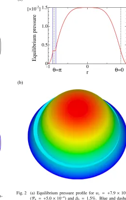
ι(1)=1.8 is also employed. Figure 1 shows the magnetic surfaces and the pressure contour of an example of the equilibria including the static island. The equilibrium corresponds towi = +7.9×10⁻² or Ψb = +5.0×10⁻⁴, where wi isthe equilibrium island width normalized by the plasma ra-dius. The magnetic surfaces are plotted by tracing the field lines as explained in Ref. [14]. Figure 2 shows the equilib-rium pressure profile along the line connecting the points of (r = 1, θ = 0,z = 0) and (r = 1, θ = π,z = 0) and the bird’s eye view of the profile for wi = +7.9×10⁻²
(Ψb = +5.0×10⁻⁴). The central beta value of 1.5% and
the profile ofPsym = P0(1−r4) are assumed in this case.
The pressure profile is locally flat inside the separatrix, while the gradient is finite at the X-point and the same as that ofPsym. The equilibrium island width varies from
−10.4×10⁻²to+10.4×10⁻²for the change of the
bound-ary poloidal flux fromΨb = −1.0×10⁻³ to+1.0×10⁻³,
as shown in Fig. 3. It is noted that positive and negative values correspond to the islands with the O-point located atθ=πandθ=0, respectively, in this figure.
The NORM code solves the reduced MHD equations as an initial value problem. For each initial component of the perturbations, ˆXm,n=( ˆΨm,n,Φˆm,n,Pˆm,n), we employ the
form of ˆ
Xm,n=σf(r), (22)
whereσdenotes the sign which takes the value of+1 or
−1 and f(r) is a function with a small absolute value corre-sponding to a white noise. In this study, we utilize the form of f(r)=10−18{1−4(r−1/2)2}2. The validity of the choice
of the initial condition is confirmed by the appearance of the sufficiently long linear phase and the behavior of the nonlinear coupling in Fig. 4. The dissipation parameters of
S = 104,ν = 8.5×10⁻⁶,κ
Fig. 1 (a) Magnetic surfaces and (b) contour of constant pres-sure of the equilibrium including a static island with the mode number of (m,n) = (1,1) forwi = +7.9×10⁻² (Ψb= +5.0×10⁻⁴). Blue lines show the separatrix of the
island.
We discuss the effect of the equilibrium island on the linear stability firstly. Figure 4 shows time evolutions of the kinetic energy for the equilibria without the island cor-responding towi=0 (Ψb=0) andσ= +1 and with the
is-land corresponding towi= +2.8×10⁻²(Ψb= +5.0×10⁻⁵)
andσ = +1. The linear phase appears in the whole range ofΨb =−1.0×10⁻³to+1.0×10⁻³, where the (m,n)=(1,1)
component is dominant. The relation of the linear growth rates among the components is different between the cases withwi=0 andwi 0. The growth rate ofEKn,nincreases
as the mode number becomes large in the case ofwi =0,
while the growth rate of each mode number is almost the same in the case ofwi 0. As is explained in Ref. [7],
this feature forwi 0 is attributed to the fact that the
(m,n) =(1,1) component is dominant and the relation of
|ΨˆJ1,1| |Ψˆ1,1|is satisfied in the linear phase.
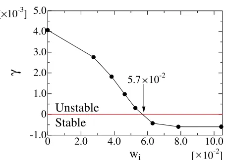
Figure 5 shows the dependence of the growth rate
Fig. 2 (a) Equilibrium pressure profile forwi = +7.9×10⁻² (Ψb = +5.0×10⁻⁴) andβ0 = 1.5%. Blue and dashed lines indicate the positions of the separatrix of the island atθ=πand the positions of the rational surface, respec-tively. (b) Bird’s eye view of the pressure profile.
γ on wi. The growth rate γ is decreased as wi is
in-creased, and the interchange mode is completely stabi-lized when wi exceeds a threshold value. The threshold
island width for the marginal stability is|wi|=5.7×10⁻²
(|Ψb|=2.3×10⁻⁴) in the present case. In the decrease of
the growth rate, the mode structure of the stream function ˆ
Φ1,1hardly changes as shown in Fig. 6. The half-width of
the modewHis 6.5×10⁻²forwi=0 (Ψb=0) and 6.6×10⁻²
forwi = +4.6×10⁻² (Ψb = +1.5×10⁻⁴). Therefore, the
threshold island width is 0.88 ofwHof the stream function
forwi = 0 (Ψb =0). Whenσis changed, the sign of the
eigenfunctions becomes opposite while the growth rate is the same. This linear stability dependence onwiimplies
curva-Fig. 3 Dependence of island width onΨb. Positive and
nega-tive values correspond to the island with the O-point at
θ=πandθ =0, respectively. Blue circles and squares showwiand the threshold width for the marginal stabil-ity, respectively. Red circles and green triangles show the island width in the saturation of interchange modes,ws, forσ= +1 andσ=−1, respectively.
Fig. 4 Time evolution of the kinetic energy for (a)wi=0 (Ψb=
0) andσ= +1 and (b)wi= +2.8×10⁻²(Ψb= +5.0×10⁻⁵)
andσ= +1.
Fig. 5 Dependence of the growth rate of the interchange mode in the linear phase onwi.
Fig. 6 Normalized ˆΦ1,1forwi=0 (Ψb=0) andwi= +4.6×10⁻² (Ψb= +1.5×10⁻⁴). Dashed line indicates the position of
the rational surface. Vertical black solid lines indicate the positions corresponding to the half value of the normal-ized ˆΦ1,1forΨb=0.
4. Nonlinear
Interaction
between
Static Magnetic Islands and
Resis-tive Interchange Modes
As shown in Fig. 4, a steady state appears after the linear phase in the time evolution of the interchange mode when the mode is unstable. Thus, we discuss the behav-ior of the interchange mode and the changes of the is-land width and the pressure profile in the nonlinear steady state. The steady state is identified with the condition of
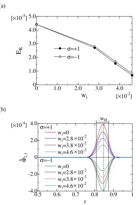
|γ| < 10−5. Figure 7 (a) shows the dependence of the
to-tal kinetic energyEK in the steady state onwi. Aswi is
increased,EKis decreased. This dependence is similar to
that of the linear growth rate shown in Fig. 5. That is, the slow growth of the mode leads to a low saturation level. Figure 7 (b) shows the profile of ˆΦ1,1 in the steady state.
Aswiis increased, the absolute value of ˆΦ1,1is decreased,
while the half-width is almost constant forwi. Therefore,
the decrease ofEKin the steady state is attributed to the
de-crease of the absolute value of ˆΦ1,1. This tendency seems
to be consistent with the experiment [2] that the fluctuation amplitude is decreased with the increase of the RMP.
Fig. 7 (a) Dependence of the kinetic energy onwi, and (b) pro-files of ˆΦ1,1in the steady state. Vertical black solid lines indicate the positions corresponding to the half value of
ˆ
Φ1,1in the steady state forwi=0.
We analyze the behavior of the island due to the non-linear evolution of the interchange mode. Before the dis-cussion for the case of the finitewi, we examine the change
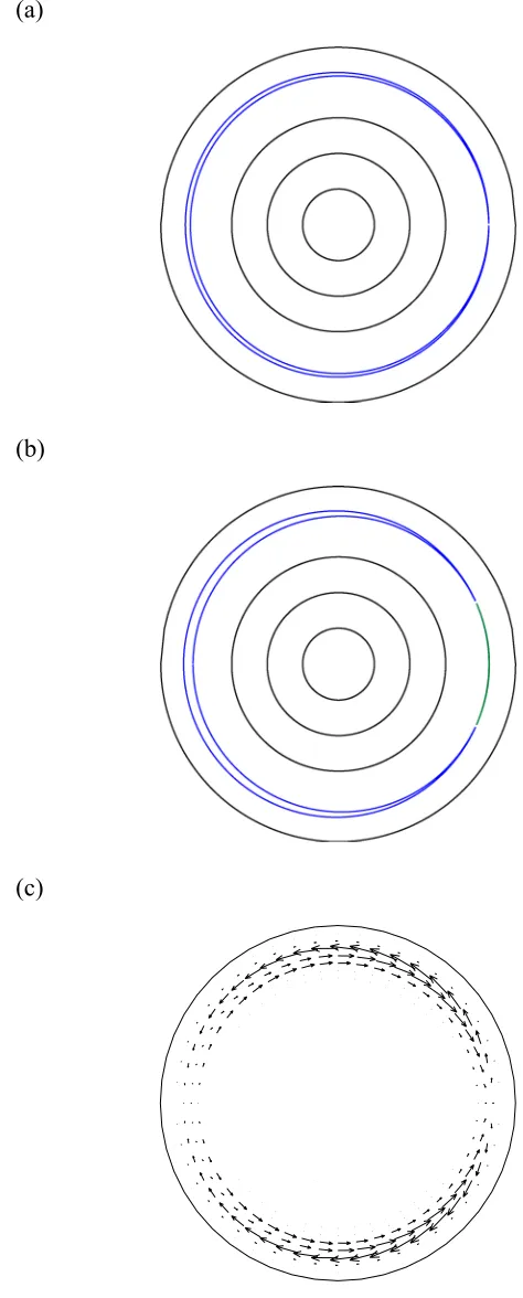
of the magnetic island in the case ofwi = 0 (Ψb = 0) as
a reference. Figure 8 (a) shows the magnetic surfaces for wi = 0 (Ψb = 0) and σ = +1 att = 10000τA. Since
we employ a large resistivity ofS = 104 in the present
analysis, the interchange mode generates a magnetic island with a substantial width even in the case ofwi =0. In the
present choice of the dissipation parameters, there are two O-points atθ=0 andθ=π, which are shown by the green and the blue lines, respectively. That is, the separatrix is composed of the mixed islands of them=1 and them=2 components. However, the island width with the O-point located atθ=πis+5.2×10⁻²and the other is−5.8×10⁻³.
Therefore, the island with the O-point located atθ =πis much larger than that with the O-point located atθ = 0. This means that them = 1 island is dominant. Thus, we neglect the smaller island and regard the separatrix as the
m =1 island. And hereafter, we refer the O-point of the
smaller island as the X-point of the larger island. The flow pattern of the vortex calculated from ˜Φatt =10000τAis
also plotted in Fig. 8 (b). This flow shows a typical pattern of anm=1 interchange mode. The influence of them=2 component to the flow is too small to be recognized. Thus, the flow pattern also validates the neglect of them = 2 component. There exist the outward and the inward radial flows at the X-point ofθ = 0 and the O-point ofθ = π, respectively. The directions of the flow is consistent with the reconnection at the X-point. In the case ofσ=−1, the phase of the magnetic surfaces and the flow are opposite to those ofσ= +1.
Next, we discuss the case of wi 0 (Ψb 0). The
magnetic surfaces att =0 andt =14000τAare shown in
Figs. 9 and 10. The separatrix is composed of the mixed islands of them = 1 and the m = 2 components in the magnetic surfaces at t = 14000 in both cases as in the case ofwi = 0. We also neglect the m = 2 component
and regard the separatrix as them=1 island. In the case of wi = +2.8×10⁻² (Ψb = +5.0×10⁻⁵) and σ = +1,
the island width is increased by the nonlinear evolution of the interchange mode as shown in Fig. 9. In the case of wi = +2.8×10⁻² (Ψb = +5.0×10⁻⁵) andσ = −1, the
island phase is changed by the interchange mode as shown in Fig. 10.
The island width in the steady state, ws, is
summa-rized in Fig. 3. Red circles and green triangles show the width for σ = +1 and σ = −1, respectively. Blue squares show the threshold width for the marginal stability (wi = +5.7×10⁻²). The island width changes only in the
region of|wi| ≤5.7×10⁻², because the interchange mode
is stable outside the region. In the region|wi|<5.7×10⁻²,
there are two cases in the island change depending onσ. One is the increase of the island width and the other is the decrease of the width as in the study of Ref. [7]. In the latter case, the island phase can also be changed. Fig-ures 9 and 10 are the examples of the former and the latter changes, respectively. These changes are attributed to the fact that the island width in the steady state is determined by the superposition of the island generated by the non-linear evolution of the interchange mode and the equilib-rium magnetic island. The island width is increased if the phase of the equilibrium island is the same as that of the island generated by the interchange mode, and decreased if opposite. The phase of the island generated by the in-terchange mode depends onσ. Therefore, the two kinds of change in the island width occur depending onσ. The flow patterns of the two cases are also plotted in Fig. 9 (c) and Fig. 10 (c). The island width increases when the flow di-rection is radially outward at the X-point of the equilibrium island. The island width decreases and the island phase can change when the flow direction is radially inward at the X-point. The radially outward shift of the plasma compresses the magnetic surfaces, which enhances the reconnection of the field lines. Therefore, the radial direction of the flow is consistent with the driven reconnection of the field lines.
Fig. 9 Magnetic surfaces at (a)t=0 and (b)t=14000τAand (c) flow pattern att = 14000τA forwi = +2.8×10⁻² (Ψb= +5.0×10⁻⁵) andσ= +1.
Fig. 10 Magnetic surfaces at (a)t=0 and (b)t=14000τAand (c) flow pattern att = 14000τA forwi = +2.8×10⁻² (Ψb= +5.0×10⁻⁵) andσ=−1.
0,z=0) and (r=1, θ=π,z=0) att=0 andt=10000τA
forwi=0 (Ψb =0) andσ=±1. Them=1 deformation
due to the interchange mode around the resonant surface
Fig. 11 Profiles of pressure (a) along the line connecting (r = 1, θ = 0,z = 0) and (r = 1, θ = π,z = 0) and the enlargements at (b)θ = 0 and (c)θ = πforwi = 0 (Ψb=0) andσ=±1. Black solid lines show the
equi-librium pressure profile. Red and green solid lines show the pressure profiles in the steady state (t= 10000τA) forσ= +1 andσ=−1, respectively. Vertical dashed lines indicate the positions of the rational surface.
Fig. 12 Profiles of pressure (a) along the line connecting (r = 1, θ=0,z=0) and (r=1, θ=π,z=0) and the enlarge-ments at (b)θ=0 and (c)θ=πforwi = +2.8×10⁻² (Ψb = +5.0×10⁻⁵) and σ = ±1. Black solid lines
show the equilibrium pressure profile. Red and green solid lines show the pressure profiles in the steady state (t =14000τA) forσ = +1 andσ = −1, respectively. Vertical dashed lines indicate the positions of the ratio-nal surface.
lower pressure at the outside of the surface is convected to the inside of the surface atθ = π. As a result, the pres-sure is increased at the X-point of the generated island and decreased at the O-point. This mechanism is the same for σ=−1.
This mechanism is also the same in the finitewicase.
Figure 12 shows the pressure profiles forwi= +2.8×10⁻²
(Ψb= +5.0×10⁻⁵) andσ=±1. The change of the pressure
is due to the convection of the radial flow as in the case of wi =0. It is remarkable that the local flat structure at the
O-point of the equilibrium island or atθ=πremains even in the saturation phase in either value ofσ. Particularly, in the case ofσ =−1, the pressure is increased atθ = π with the local flat structure kept in spite of the fact that the point is changed to the X-point from the O-point as shown in Fig. 10. Therefore, the nonlinear saturation of the inter-change mode does not reproduce a new equilibrium with a pressure profile corresponding to the resultant magnetic islands.
5. Conclusions
The effects of the (m,n) = (1,1) static magnetic is-land on the resistive interchange mode with the same mode number are studied. For this purpose, we utilize equilibria with the pressure profile consistent with the island geome-try of which the gradient at the X-point is finite. The lin-ear growth rate of the interchange mode is reduced by the equilibrium island in spite of the finite pressure gradient at the X-point. Beyond a threshold island width, the mode is completely stabilized. The threshold width is almost the same as the half-width of the stream function obtained for the equilibrium without the island. The effect of the static island on the interchange mode can be observed in RMP experiments by detecting both the width of the flat region in the pressure profile data and the fluctuation amplitude resonant at the surface of the island. The stabilizing ten-dency and the existence of the threshold width obtained in the present analysis is consistent with the experimental results in LHD [2]. More quantitative comparison will be planed in future.
In the nonlinear saturation phase of the unstable in-terchange mode, the saturation level of the kinetic energy is also decreased as the island width is increased. On the other hand, the nonlinear evolution changes the shape of the magnetic island. If the phase of the equilibrium island is the same as that of the island generated by the inter-change mode, the island width is increased. If the phase is opposite, the island width is decreased and the phase can also be changed. In the point of the relation with the flow generated by the mode, the island width increases when the flow direction is radially outward at the X-point of the initial static island and decreases when the flow direction is radially inward at the X-point. The interchange mode also changes the pressure profile through the convection. The tendency of the profile change is almost independent of the equilibrium island structure. The pressure is increased and decreased by the outward and the inward flows, respec-tively. The local flat structure at the O-point of the static island is almost kept even if this point is changed to the X-point.
uni-form poloidal flow such as a diamagnetic flow. If the effect is included, the interchange modes are possible to rotate. Then, the static island with a substantial width may lock the mode rotation. Such mode locking was discussed in Ref. [9] with a smooth equilibrium pressure profile. By utilizing the local flat equilibrium pressure consistent with the island structure, the mode locking due to the static is-land can be investigated more consistently.
Another future work is the change of the Fourier mode of the perturbation. In the present analysis, we focus on the interaction between the static island and the interchange mode with the same mode numbers, (m,n) = (1,1). For this purpose, we adjust the dissipation parameters so that the (1,1) component of the interchange mode should be dominant. By choosing appropriate dissipation parame-ters, we can set the dominant mode numbers to higher numbers, such as (2,2), (3,3) and so on. It is interesting to analyze the change of the (1,1) island structure due to the dynamics flow with such high mode numbers. On the other hand, the interaction between the islands with higher mode numbers of (2,2), (3,3) and so on and the (1,1) in-terchange mode is considered as another research aspect. Also in this case, the islands make the equilibrium pres-sure profile locally flat. Therefore, it is expected that the islands essentially have a stabilizing contribution to the in-terchange mode as well. However, further calculations are needed to obtain the quantitative stabilizing property.
Including the multi-helicity perturbation should also be considered. Local flattening of the pressure profile makes the pressure gradient steeper in the region just out-side the separatrix. Therefore, the interchange mode reso-nant at the region can be destabilized. Since such a mode has a helicity different from that of the static island, the multi-helicity perturbations are needed to analyze the ef-fect of the static island on the interchange stability in the whole plasma.
Acknowledgments
This work is partly supported by the budget NIFS11KNXN222 of National Institute for Fusion Science and by JSPS KAKENHI Grant Number 22560822.
[1] M.E. Fenstermacher, M. Becoulet, P. Cahyna, J. Canik, C.S. Chang, T.E. Evans, P. Gohli, S. Kaye, A. Kirk, Y. Liang, A. Loarte, R. Maingi, O. Shmitz, W. Suttrop and H.R. Wilson, Proceedings of 23rd IAEA Fusion Energy Conference, 11-16 October 2010, Daejeon, Republic of Korea, ITR/P1-30.
[2] H. Yamada, K.Y. Watanabe, S. Sakakibara, Y. Suzuki, S. Ohdachi, M. Kobayashi, H. Funaba and the LHD Exper-imental Group, Contrib. Plasma Phys. 50, No.6-7, 480 (2010).
[3] A. Komori, H. Yamada, O. Kaneko, K. Kawahata, T.
Mutoh, N. Ohyabu, S. Imagawa, K. Ida, Y. Nagayama, T. Shimozuma, K.Y. Watanabe, T. Mito, M. Kobayashi, K. Nagaoka, R. Sakamoto, N. Yoshida, S. Ohdachi, S. Sakakibara, N. Ashikawa, Y. Feng, T. Fukuda, H. Igami, S. Inagaki, H. Kasahara, S. Kubo, R. Kumazawa, O. Mitarai, S. Murakami, Y. Nakamura, M. Nishiura, T. Hino, S. Masuzaki, K. Tanaka, K. Toi, A. Weller, M. Yoshinuma, Y. Narushima, N. Ohno, T. Okamura, N. Tamura, K. Saito, T. Seki, S. Sudo, H. Tanaka, T. Tokuzawa, N. Yanagi, M. Yokoyama, Y. Yoshimura, T. Akiyama, H. Chikaraishi, M. Chowdhuri, M. Emoto, N. Ezumi, H. Funaba, L. Garcia, P. Goncharov, M. Goto, K. Ichiguchi, M. Ichimura, H. Idei, T. Ido, S. Iio, K. Ikeda, M. Irie, A. Isayama, T. Ishigooka, M. Isobe, T. Ito, K. Itoh, A. Iwamae, S. Hamaguchi, K. Hamajima, S. Kitajima, S. Kado, D. Kato, T. Kato, S. Kobayashi, K. Kondo, S. Masamune, H. Matsumoto, N. Matsunami, T. Minami, C. Michael, H. Miura, J. Miyazawa, N. Mizuguchi, T. Morisaki, S. Morita, G. Motojima, I. Murakami, S. Muto, K. Nagasaki, N. Nakajima, Y. Nakamura, H. Nakanishi, H. Nakano, K. Narihara, A. Nishimura, H. Nishimura, K. Nishimura, S. Nishimura, N. Nishino, T. Notake, T. Obana, K. Ogawa, Y. Oka, T. Ohishi, H. Okada, K. Okuno, K. Ono, M. Osakabe, T. Osako, T. Ozaki, B.J. Peterson, H. Sakaue, M. Sasao, S. Satake, K. Sato, M. Sato, A. Shimizu, M. Shiratani, M. Shoji, H. Sugama, C. Suzuki, Y. Suzuki, K. Takahata, H. Takahashi, Y. Takase, Y. Takeiri, H. Takenaga, S. Toda, Y. Todo, M. Tokitani, H. Tsuchiya, K. Tsumori, S. Urano, E. Veshchev, F. Watanabe, T. Watanabe, T.H. Watanabe, I. Yamada, S. Yamada, O. Yamagishi, S. Yamaguchi, S. Yoshimura, T. Yoshinaga and O. Motojima, Proceedings of the 22nd Fusion Energy Conference OV/2-4 (2008). [4] T. Unemura, S. Hamaguchi and M. Wakatani, Phys.
Plas-mas11, 1545 (2004).
[5] L. Garcia, B.A. Carreras, V.E. Lynch, M.A. Pedrosa and C. Hidalgo, Phys. Plasmas8, 4111 (2001).
[6] L. Garcia, B.A. Carreras, V.E. Lynch and M. Wakatani, Nucl. Fusion43, 553 (2003).
[7] K. Saito, K. Ichiguchi and N. Ohyabu, Phys. Plasmas17, 062504 (2010).
[8] K. Saito, K. Ichiguchi and R. Ishizaki, Plasma Fusion Res.
6, 2403072 (2011).
[9] S. Nishimura, K. Itoh, M. Yagi, K. Ida and S.-I. Itoh, Phys. Plasmas17, 122505 (2010).
[10] S. Nishimura and M. Yagi, Plasma Fusion Res.6, 2403119 (2011).
[11] S. Nishimura, S. Toda, Y. Narushima and M. Yagi, Plasma Phys. Control. Fusion, in press, (2012).
[12] H.R. Strauss, Plasma Phys.22, 733 (1980).
[13] K. Saito, K. Ichiguchi and R. Ishizaki, Plasma Fusion Res.
7, 1403070 (2012).
[14] K. Saito, K. Ichiguchi and R. Ishizaki, Plasma Fusion Res.
7, 2403032 (2012).
[15] K. Ichiguchi, N. Nakajima, M. Okamoto, N. Ohyabu, T. Tatsuno, M. Wakatani and B.A. Carreras, J. Plasma Fusion Res. SERIES2, 286 (1999).
[16] K. Ichiguchi, M. Wakatani, T. Unemura, T. Tatsuno and B.A. Carreras, Nucl. Fusion41, 181 (2001).