Dynamic Output Feedback Control for Nonlinear Uncertain Systems with Multiple Time-Varying Delays

http://www.sciencepublishinggroup.com/j/acis doi: 10.11648/j.acis.20180601.12

ISSN: 2328-5583 (Print); ISSN: 2328-5591 (Online)

Dynamic Output Feedback Control for Nonlinear Uncertain

Systems with Multiple Time-Varying Delays

Wei Zheng

1, *

, Hongbin Wang

1

, Zhiming Zhang

2

, Pengheng Yin

1 1

Institute of Electrical Engineering, Yanshan University, Qinhuangdao, China 2_{China National Heavy Machinery Research Institute, Xi'an, China}

Email address:

*

Corresponding author

To cite this article:

Wei Zheng, Hongbin Wang, Zhiming Zhang, Pengheng Yin. Dynamic Output Feedback Control for Nonlinear Uncertain Systems with Multiple Time-Varying Delays. Automation, Control and Intelligent Systems. Vol. 6, No. 1, 2018, pp. 8-19. doi: 10.11648/j.acis.20180601.12

Received: December 26, 2017; Accepted: January 25, 2018; Published: April 2, 2018

Abstract:

This paper addresses the adaptive dynamic output-feedback control problem for a class of nonlinear discrete-time systems with multiple time-varying delays. First, the guaranteed cost function is introduced for the nonlinear system to reduce the effect of the time-varying delays. Secondly, in order to deal with the multiple time-varying delays, the nonlinear system is decomposed into two subsystems. Then the compensator is designed for the first subsystem, and the adaptive dynamic output-feedback controller is constructed based on the subsystems. By introducing the new discrete Lyapunov-Krasovskii functional, it can be seen that the solutions of the resultant closed-loop system converge to an adjustable bounded region. Finally, the simulations are performed to show the effectiveness of the proposed methods.

Keywords:

Multiple Time-Varying Delays, Parametric Uncertainties, Dynamic Output Feedback Control, Lyapunov-Krasovskii Functional

1. Introduction

Many practical systems are the nonlinear systems and consist of time-delay, such as the urban traffic networks system, digital communication system, and the power systems [1-3]. As universal approximators, fuzzy systems or neural networks have been successfully applied to solve the control design problem for various kinds of such nonlinear systems, and many interesting results have been obtained see [4-6] and the references therein. It is noted that with those control schemes, the stability of the closed-loop systems can be guaranteed, and the tracking errors can be confined to a small residual set, while the size of the residual sets is often unknown, and the transient and/or steady state performance cannot be prescribed.

The Lyapunov-Krasovskii functional method and

Lyapunov-Razumikhin method are always employed for the system design. In recent years, many adaptive fuzzy/neural output-feedback control approaches have been proposed for uncertain SISO/MIMO nonlinear systems with unmeasured states in [7, 8]. Note that all the aforementioned adaptive fuzzy/neural output-feedback control schemes are for the

nonlinear strict-feedback uncertain systems [9], instead of the nonlinear nonstrict-feedback ones [10, 11]. In [12], the robust-control problem for the time-delay systems was considered, and the nonlinear uncertainties are bounded by the high-order polynomials. A tracking control system has a more general form than a general nonlinear system, and yet the system functions contain the whole state variables [13, 14]. But how to apply this method into the nonlinear time-delay systems is a challenging subject [15]. By employing the neural network technique, the state feedback controller is designed for the time-delay nonlinear systems. Compared with the previous work, in the effort to develop new adaptive control strategies, adaptive neural back-stepping state feedback control methodologies for nonlinear systems were proposed in [18]. There are few results on dynamic output feedback control for nonlinear system with time delays

methods were proposed for the robotic system.

Based on the neural networks, a robust adaptive control method for a class of uncertain nonlinear systems in the presence of input saturation and external disturbance was proposed [21]. And an adaptive tracking control was designed for a class of uncertain multi-input and multi-output nonlinear systems with non-symmetric input constraints by using an auxiliary system [22]. Then, the input saturation problem was investigated for stochastic nonlinear systems [23]. In [24], the output feedback control problem for identical linear dynamic systems with input saturation was addressed. To our best knowledge, there are no results on output feedback control results for feedback nonlinear systems with time-delays and multiple subsystems.

In this paper, the dynamic output feedback control approach is proposed for the mobile robot system with multiple time-varying delays. The contributions of this paper can be summarized as follows:

(1) The cost function is introduces to deal with the time-delays.

(2) The nonlinear system is decomposed into two subsystems based on the input matrix and output matrix. The dynamic compensator is developed for the first subsystem. And the dynamic output-feedback controller is designed based on the second subsystem.

(3) By introducing the new Lyapunov-Krasovskii functional, it can be seen that the solutions of the resultant closed-loop system converge to an adjustable bounded region. This paper is organized as follows. The preliminary knowledge for the nonlinear multiple time-varying delays system with parametric uncertainties are described in Section 2. The dynamic output-feedback controller for the nonlinear system is designed in Section 3. The results are further extended to the general nonlinear discrete-time case in Section 4. The simulation results are performed for a mobile robot case in Section 5. Finally, Section 6 concludes with a summary of the obtained results.

The rest of paper is organized as follows. Section 2 presents some preliminary knowledge for the dynamicsystem with. In

Section 3, the dynamic output-feedback controller is presented. The proving process is shown in Section 4. The simulation results are presented in Section 5. Finally, Section 6 concludes with a summary of the obtained results

2. System Formulation and Preliminaries

Consider a nonlinear discrete system with multiple time-varying delays and parametric uncertainties as follows.

0

1 2

( ) ( ) ( ( )) ( ( )

( ( ), ( ( )), ( ( )), , ( ( ))))

( ) ( )

1

…

r

j j j

j

r

k

x = A A x k - k B u k

f x k x k - k x k - k x k - k y = C kx

+

k

τ

τ τ τ

=



∑ + ∆ +

 

+

   

(1)

where x k( )∈Rn is the state variable, ( )u k ∈Rm is the control

input, and y k( )∈Rp is the control output. Aj Rn n

×

∈ ,

n m

B∈R × and C∈Rp n× are gain matrices with appropriate

dimensions, ∆ ∈Aj Rn n× are the unknown matrix representing

the parametric uncertainties. τj( )k are the multiple

time-varying delays satisfies 1>τ∗j≥τj(k+1) and τj≥τj( )k ,

where

τ

0( )=0k , τj ∗

and

τ

j are the positive scalars. The

nonlinear function _f( )i _{is uncertain and contains multiple}

time-varying delays.

Assumption 1. For the nonlinear function _f( )i _{, the}

following inequality holds

0

1 2

( ( ( )) )

( ( ), ( ( )), ( ( )),…, ( ( )))

r T

j j j

j

r

x k k

f x k x k k x k k x k k

ϑ α τ

τ τ τ

=

∑ −

≥ − − −

(2)

where ϑj∈Rpj is unknown constant vector.

1 2

( )i [ ( ),i ( ),i …, ( )]i T

j j j ji

α = α α α , αji is known function with

(0) 0

ji

α

= . And there exist the nonlinear functions ( )i

ji

α

satisfying xαji( )x ≥αji( )x .

Remark 1. In this paper, the adaptive control theory was presented to estimate the system parameters or uncertain bound parameters. In [25], the adaptive control theory was discussed with some unknown interconnections. Since the research contains the nonlinear functions, it can be seen that the schemes are not enforceable to system (1). In this paper, there are three challenging problems as follows: how to design a dynamic compensator with the output feedback signal; how to reduce the influence of uncertain parameters; and how to design the adaptive output feedback controller for the multiple time-delays system. The aim of this paper is to solve the above issues, and then the controller will be easy to implement in practical systems.

In this paper, 0_{( )}

T m m n-m m

B=_{ ×} B _× _ and C=_0_{( )n- p×p} D_{p p×} _T,

where Bm m× and D satisfying Rank B( m m× )=m and

m U

T T

DD =D D= , Um is the identity matrix. Let

1 2 T T x x

x

 

= 

 

 ,

then the system (1) is rewritten as follows:

1 12 12 2

0

11 11 1

2 22 22 2

0

21 21 1

1

1

2

( 1) (( ) ( ( ))

+( ) ( ( )))

( 1) (( ) ( ( ))

+( ) ( ( )))

+ ( ( ), ( - ( )), , ( - ( ))) ( )

( )

… r

j j j

j

j j j

r

j j j

j

j j j

r T

T

x k A A x k - k

A A x k - k

x k A A x k - k

A A x k - k

Bf x k x t k x k k Bu k

x y k C

x

τ τ

τ τ

τ τ

=

=



+ = ∑ + ∆

 

 _{+ ∆}



 _{+ = ∑ + ∆}

 

+ ∆

 

+



 _{ }

 _{=  }

 _{ }

 



(3)

matrices of Aj . ∆Aj11 , ∆Aj12 , ∆Aj21 and ∆Aj22 are the

decomposition matrix of ∆Aj. With m< p, one has 1

2 T T y y

y

 

= 

 

 .

For the matrices _B and _C , there exist the nonsingular

matrices _E∈Rm m× _{and C}ɶ_∈R( - )( - )p m n m _satisfying

1 1

ɶ

y =Cx and

2 2

y =Ex .

With the above analysis, the system (1) is further rewritten as follows:

1 11 11 1

0

12 12 2

2 21 21 1

0

22 22 2

1 1

2

( 1) (( ) ( ( ))

( ) ( ( )))

( 1) (( ) ( ( ))

( ) ( ( )))

+ ( ( ), ( - ( )), , ( - ( )))+ ( ) ( )

( ) ( )

… ɶ

r

j j j

j

j j j

r

j j j

j

j j j

r T

T

x k A A x k - k

+ A A y k - k

y k A A x k - k

+ A A y k - k

EBf x k x k k x k k EBu k Cx

y k Ex

τ

τ

τ

τ

τ τ

=

=



+ = ∑ + ∆

 

 _{+ ∆}

 

+ = ∑ + ∆

 

+ ∆

 

= 

 

 

       

(4)

where Aj11=Aj11 ,

1

12 12

j j

A =A E− , Aj21=EAj21 , 1

22 22

j j

A =EA E− , ∆Aj11= ∆Aj11 ,

1

12 12

j j

A A E−

∆ = ∆ ,

21 21

j j

A E A

∆ = ∆ and ∆Aj22= ∆E Aj22E−1.

3. Controller Design

First, a cost function is introduced for the nonlinear system

to deal with the uncertain parameters ∆A_j . Secondly, a

dynamic compensator is designed for the subsystem-x1, and

the adaptive output-feedback controller is constructed base on

the second subsystem-y2 and the compensator.

3.1. Cost Function Design

In this study, the uncertainties are norm-bounded, described as follows:

[

]

11 12

1 2

21 22

( )

j j

j j

A A

M k Q Q

A A

∆ ∆

 

=

 

∆ ∆

 

 

where Q1 and Q2 are the constant matrices, M k( ) is an

unknown matrix satisfying MT( )k M k( )≤U_m . Let

1

0< ∈λ Rn n× and 0 2

m m R

λ ×

< ∈ . Consider the cost function

for the system (1) as follows

1 2

0

[ T( ) ( ) T( ) ( )]

t

J ∞ x k

λ

x k u k

λ

u k =

= ∑ + (5)

Now, in order to improve the stability of system (3), one has

ˆ( 1) ˆ( ) ( ), (0)ˆ 0 ˆ

( ) ( )

c c

c

x k A x k B y k x u k C x k

+ = + =

= (6)

where x kˆ( ) is the state vector. Then applying (6) to the system (3), the new closed-loop system is obtained as follows

2 0

( 1) ( _j ( ) ) ( ) r ( _j ( ) ) ( _j( ))

j

x k A M k Q x k A M k Q x k τ k

=

+ = + + ∑ _{+ − (7)}

where

( ) ( )

ˆ( ) x k x k

x k

 

= 

 ,

j c

j

c c

A BC A

B C A

 

= 

 

 , Q=Q1 Q C2 c

For the closed-loop system (7), design the cost function as follows

0

( ) ( )

T

t

J x k

λ

x k ∞

=

= ∑ (8)

where λ=diag[ ,λ₁ C_cTλ₂C_c].

With the cost function (5), the Assumption 2 is imposed on system (3):

Assumption 2. Consider the nonlinear system (3) and cost function (5), the initial states of system (3) are given. If there exist the equation (6) and a positive scalar J∗ such that

J≤J∗, then the closed-loop system is stable.

Lemma 1. [26]: Let Jˆ=JˆT >0, mˆ₁, mˆ₂ are the known matrices with appropriate dimensions. Then the following inequalities hold:

1

1 1 2 2

ˆ _{ˆ ˆ}T _{ˆ ˆ}T ₀

J+

ϖ

−m m +

ϖ

m m <

1 2 2 1

ˆ _{ˆ ˆ ˆ}T T _ˆT ₀

J+m Mm +m M m <

where M MT ≤U_m and ϖ is a positive scalar.

Lemma 2. [27]: For matrices n₁>0 and n₂ >0, if there exist a matrix Θ such that Θ = Θ >T 0, then the following inequality holds:

1

1 2 1 1 2 2

2n nT nT n nT −n

− ≤ Θ + Θ .

3.2. Compensator Design

For subsystem-x k1( +1), the augmented dynamic system is

designed as follows:

( )

( )

( )

(

)

( )

( )

2 1

1 1

l l

l l

y k C k D y k k A k B y k

ζ

ζ ζ

 _{= +}

 

+ = +

 (9)

where ζ∈Rn m− , _y2

( )

_{k ∈R}m_{, , ,}

l l l

A B C and D_l are designed with appropriate dimensions. With equations (4) and (9), one has:

(

)

(

( )

)

( )

1 1

r

j j

j

k N k k I k w

δ δ τ δ

=

where 12

(

( )

)

0

r

j j

j

w A z k τ k

=

= ∑ − in which

( )

2

( )

2

( )

z k =y k −y k ,

( )

k x k1

_{( )}

( )

k δ ζ   =     ,

011 012 012

ɶ ɶ

l l

l l

A A D C A C

I

B C A

 ₊ 

= 

 

  and

11 12 12

0 0

ɶ

j j l j l

j

A A D C A C

N

 ₊ 

= 

 

 

For equation (10), choose a discrete Lyapunov-Krasovskii functional as follows:

( ) ( )

( )

( )

( ) ( )

( )

_{( )}

_{( )}

1 1 0 1 ɺ ɺ j j

r _{c k}

k T

j k k

j

r _{c k}

T k T

k j

j

V e R d

k P k e Z d d

σ τ σ τ θ δ σ δ σ σ δ δ δ σ δ σ σ ϑ − − = − − + = =∑ + +∑

∫

∫ ∫

(11)

where P R, _j, and Z_j are the positive matrices, c and σ are the positive scalars. Now taking the forward difference of (11), one has:

(

)

(

)

(

( )

( )

( )

)

( )

( )

(

)

(

( )

(

)

(

( )

)

)

( ) (

)

( ) ( )

1 1 1 1 1 1 1 2 1 ɺ ɺ j j j r T j j j c k T j k k r T j j j c T

j j j

T T

V k Z k

e Z d

k R k

e k k R k k

cV k P k c k P k

τ τ τ τ δ δ δ σ δ σ σ δ δ τ δ τ δ τ δ δ δ δ = − − ∗ = − ∆ ≤ ∑ _{+ +} − +∑ _{− −} × − − − + + +

∫

(12) Note that:

( )

(

)

( )

_{( )}

( )

_{( )}

( )

(

( )

)

(

)

1 1 0

2 T T

0

ɺ

i

r r

T T

j ij i r

i j

k

i k k

k k w k

k _τ d k k

δ τ δ δ σ σ δ τ + = = −   ∑ ∑_{ − + }   × −

∫

− − = (13)

where T_ij is a weight matrix. With equations (10), (12) and (13), one has:

( )

( ) ( )

2 1 1 1 , , i r

T k T

i k k

i

V ε w cV a Ga _−τ x kζ F x kζ ζd

=

∆ ≤ − + +∑

∫

₍₁₄₎

where a _and ε _{are the positive scalars,} T

T i

i i i T c

i i

X F

e−τZ

 

= 

−

 

  with

( ) ( )2 2

i ilj _{r r}

X X

+ × +

 

=_{  , ( )}

0 1

T T ⋯ T

T

T T

i = −_ i − i r+ _ . G is defined

as follows:

(

)

11 0 0 11

1 1 T T 1 1

r r r r

T T T

i i i i i i j

i i i j

G τI Z I PI I P cP τX R

= = = =

= Σ + + Σ + + + − Σ + Σ ,

( ) ( )

1 ₁ 1 1 ₁ 1 T 1 0 ₁T 1

r r r

T T

j _i i i j j _i i i j j _i i j

G τ I Z N₋ PN ₋ τ X _{− −}

= = =

= Σ + − Σ − + Σ for

1 2

r+ ≥ ≥j ; _{1( )2 ( )1 1( )2}

1T 1 1

r r r

T T

i i i

r _i i r _{i i} i r

G _{+ +} τ I Z τ X ₊ P

= = =

= Σ + Σ − Σ ,

1 ( 1)( 1)

1 1 1 ( 1)( 1)

1 1

T j T

j j

r r _c

T T

jj i j i j i ijj j j j

i i

G τN Z N τ X e τ−R

− −

−

− − − − −

= =

=∑ ₋∑ _{− − −}

for r+ ≥ ≥1 j 2 ;

( )( ) ( )( )

1 1 1 1 1 1

1 1

T T

r r

T T

jq i j i q i ijq j q q j

i i

G τN ₋Z N ₋ τ X _{− − − −}

= =

= Σ − Σ − − for

1 1

r+ ≥ ≥ +q j _{; ( )2 ( )2 ( )( )1 1 1}

1 1

T

r r

T T

i i j i

j r ij r j r

i i

G ₊ τ X _{+ − +} τN ₋Z

= =

= −∑ _{− +}∑

for r+ > >1 j 2_{; ( 2)( 2) ( 2)( 2)}

1 1

U

r r

i i m i

r r i r r

i i

G _{+ +} τZ ε τ X _{+ +}

= =

=∑ − −∑ _,

( )

(

1

( )

)

⋯

(

( )

)

T

T T T T

r

a=_δ k δ k−τ k δ k−τ k w _ ,

( )

, T ɺT

( )

T

x k ζ =_a δ ζ _ and G=Gij₍r+ × +2_{) (}r 2₎.

With the above analysis, the new results arise:

Theorem 1. ∀ positive scalar ε , there exist the positive matrices P R Z, _i, _i, T_ij and Xilj such that G<0 and Fi <0

for any _i=(1, 2,…, )_{r . With Theorem 1 and (14), taking the}

forward difference of V1 along (10), one has

2

1 1

V

ε

w cV

∆ ≤ − (15)

Remark 2. The matrix T_il is employed to derive the

conservative conditions. The use details of T_il is shown in

[28, 29]. The compensator ( n−m order) is designed for

subsystem-x1. The matrices A B Cl, l, l, and Dl are designed

in (9), by letting C_l =0, the dynamic compensator (9) will become a static compensator.

Choose a new discrete Lyapunov-Krasovskii functional as follows:

( )

( ) ( )

(

)

( )

1 2

1 1 12

1

1 j 1

j

r _c

c k k

j k k j

j

V V τ∗ − eτ _−τ e δ− ε r A z σ dσ

=

= +∑ _{− ×}

∫

₊

with (15), one has:

(

)

(

( )

)

2

1 12 1

0 1

r

j j

j

V ε r A z k τ k cV

=

∆ ≤ ∑ + − − (16)

By direct verification, one can obtain

( )

2

1 1

V ε z k cV

∆ ≤ −

where

(

)

2

( )

1

(

)

2

012 12

1

1 1 1 j

r _c

j j

j

r A r eτ A

ε ε ε τ∗ −

=

≥ + +∑ _{− +}

With the above analysis and the compensator (9), the adaptive dynamic output-feedback controller will be designed in next section.

3.3. Adaptive Dynamic Output-Feedback Controller Design

Let ɶ

l l

C D C

 

( )

2

( )

2

( )

2

( )

z k =y k −y k =y − Λδ k . Since

( )

i

ji

α is a

nonlinear function, with Assumption 1, there exist the

unknown vector ϑj such that

( )

(

( )

)

(

( )

)

(

)

( )

(

)

(

( )

)

(

)

( )

(

)

(

( )

)

( )

(

)

( )

(

)

(

)

(

(

( )

)

)

( )

(

)

(

)

1 1 2 1 0 1 1 0 1 1 1 0 1 , , , ( )

( 3 3

3 )

… r r

T

j j j j

j r

T

j j j j

j

j r

T

j j j j j

j

j j

EBf x k x k k x k k

E y k k x k k

x k k E z k k

E k k

x k k E z k k

E k k

τ τ ϑ α τ τ ϑ α τ τ δ τ ϑ α τ α τ α δ τ − = − = − − = − − − ≤ ∑ _{− + −} ≤ ∑ _{− + −} + Λ − ≤ ∑ _{− + −} + Λ − (17)

With (4), one has:

(

)

(

(

( )

)

(

( )

)

)

( )

(

( )

( )

)

( )

(

( )

)

(

( )

)

(

)

22 2 21 1

0 1 1 1 1 , , , ɶ ɺ … r

j j j j

j

l l l l

r

z k A y k k A x k k

EBu k C A k B y k D Cx

EBf x k x k k x k k

τ τ ζ τ τ = + = ∑ _{− + −} + − + − + − − (18)

For subsystem-z k( ), where z k

( )

=y₂

( )

k −y₂

( )

k =y₂− Λδ

( )

k , choose a discrete Lyapunov-Krasovskii functional as follows:

( )

(

)

( ) ( )

( )

( ) ( )

(

( ) ( ) ( )

)

2 2 1 1 1 1 2

1 , ,

j j T r _b b k k

j k k j

j

V k z k z k

d

eτ _τ e σ F x z d

ϑ ϑ τ σ δ σ σ σ ∗ − ₋ ∗ − = = − + +∑ _{− ×}

∫

(19)

where Λ =Cl D Clɶ, b and d are the positive scalars,

ϑ

( )

k

is the adaptive parameter with 1

03 r T j j j ϑ∗ −ϑ ϑ =

= ∑ ϒ .

( )

i j F is

defined as:

( ) ( ) ( )

(

)

( )

(

)

( )

(

)

(

( )

)

( )

( )

( )

1 2 1 2 2 1 1

2 2 2 2

1 1 1

1 1 2 2

, , 3 3 3 j j j l

F x z

E z

E x

x z C

σ δ σ σ α σ α δ σ α σ µ σ µ σ µ ζ σ − − − − − = ϒ +ϒ Λ + ϒ + + +

where µ1 µ2 and ϒ are the positive scalars.

Now, taking the forward difference of V2 yields:

( ) ( )

(

( )

)

( )

(

)

(

)

( ) (

)

( )

(

( ) ( ) ( )

)

( )

(

)

(

( )

)

(

( )

)

(

)

2 2 2 1 1 1 1 2 1

1 2 1

( 1 , ,

, , ) j T T r _b j j j

j j j j

b

V bV bz k z k k

d

k k z k z k

d

e F x k k z k

F x k k k k z k k

τ ϑ θ ϑ ϑ ϑ τ δ τ δ τ τ ∗ ∗ − ∗ = ∆ ≤ − + + − + − + + + +∑ ₋ − − − − (20)

With (18), one has:

( ) (

)

( )

1

21 11 1

0

22 12 2

2 1

2 ( ( ) ( ( ) ( )))

+2 ( ) (( ) ( ( ))

( ) ( ( )))

ɶ

ɶ

T

T

l l l

r T

j l j j

j

j l j j

z k z k

z k EBu k EBf C A k B y k

z k A D CA x k k

A D CA y k k

ζ τ τ = + = + − + ∑ _{− −} + − − (21)

By employing (17), such that:

1 1 0 1 1 2 2 1 1 0 2 1 2 1

2 ( ) ( ( ), ( ( )), , ( ( )))

2 ( ) ( (3 ( ( )) )

(3 ( ( )) ) (3 ( ( )) ))

(3 ( ) (3 ( ( )) )

(3 ( ( )) )

(3 ( ( )) ) )

…

T

r r

T

j j j

j

j j j j

r

T

j j j j

j

j j

j j

z k EBf x k x k k x k k

z k x k k

E k k E z k k

z k x k k

E k k

E z k k

τ τ ϑ α τ α δ τ α τ ϑ ϑ α τ α δ τ α τ = − − − = − − − − ≤ ∑ − + Λ − + − ≤ ∑ ϒ + ϒ − +ϒ Λ − +ϒ − (22)

21 11 1 0

22 12 2

21 11

0

22 12 1

22 12

0

2 ( ) (( ) ( ( ))

( ) ( ( )))

2 ( ) (

( ) ) ( ( ))

2 ( ) ( ) ( ( ( )) ( ( )))

ɶ

ɶ

ɶ

ɶ ɶ

ɶ r

T

j l j j

j

j l j j

r T

j l j

j

j l j l j

r T

j l j j l j

j

z k A D CA x k k

A D CA y k k z k A D CA A D CA D C x k k

z k A D CA z k k C k k

τ

τ

τ

τ ζ τ

=

=

=

∑ _{− −}

+ − −

= ∑ ₋

+ − −

+ ∑ _{− × − + −}

(23)

By letting

2

21 ( 22 12) 11 1

ɶ ɶ ɶ

j j l j l l j

A + A −D CA D C−D CA ≤s

2

22 12 2

ɶ

j l j

A −D CA ≤s

where s1 and s2 are the transition parameters. For j∈[1, r], one has:

2

2 2

1 1

1 1 1 1 1 1

1

21 11 22 12 1

0

( ) (1 ) ( ) ( ( ))

2 ( ) ( ɶ ( ɶ ) ɶ) ( ( ))

r

j j

r T

j l j j l j l j

j

x k r s z k x k k

z k A D CA A D CA D C x k k

µ µ µ τ

τ

− −

=

=

+ + +∑ −

≥ ∑ _{− + − −}

(24)

and

2 2 2 2

1 1

2 2 2 2

1

22 12

1

( ( ( )) ( ( )) )+2 ( )

2 ( ) ( ɶ )( ( ( ))+ ( ( )))

r

j l j

j

r T

j l j l j j

j

z k k C k k r s z k

z k A D CA C k k z k k

µ τ µ ζ τ µ

ζ τ τ

− −

=

=

∑ _{− + −}

≥ ∑ _{− − −}

(25)

Design the control law u k( )=(EB)−1u k( ) for system (1) where

012 022

1

1 1

1 1

2 2 2

1

2

2 1

0

2

1 1

1

( ) ( )( ( ) ( ))

1

( ( ) ( )) ( ( ))

2

1 1

( ) ( ) (( 1)

2 2

2 (1 ) ) ( )

4.5 ( )( (3 ( ) )

(1 ) (3 ( ) ) )

ɶ

j

j

l l

l l l

r

b j j

r

b

j j

j

u k D CA A z k C k

C A k B y k z k

k z k r s b

r s e z k

E z k E z k

e E z k

τ

τ

ζ

ζ φ

ϑ µ

µ τ µ

α

τ α

∗ − −

=

− −

∗ − −

=

= − +

+ + −

− − + +

+ + ∑ ₋

− ϒ

+∑ ₋

(26)

in which

φ

( ( ))z k is a nonlinear function,

φ

( ( ))z k is employed

to reduce the influences of parameter δ in subsystem (10).

Substituting (21)–(26) into (20) yields:

2 2

2 1

( ( ) ) ( 1)

( ( )) ( ) ( ) ( ) ( ( ))

( ( )) ( ( ) )

2

T T

V k k bV

d

k z k z k z k z k b

k k

d

ϑ ϑ ϑ

ϑ ϑ φ

δ ϑ ϑ

∗

∗

∗

∆ ≤ − + −

+ − −

+Φ + −

(27)

where Φ( ( ))

δ

k is defined as follows:

( )

2 2

1

1 1 0 1

2 1

0

2 1

1 1

2 1

2 2 2

1 1 1

2 1 1

1

( ( )) ( ) (3 ( ) )

(3 ( ) )

(1 ) ( (3 )

(3 ( ) ) )

(1 ) ( ( ) ( ) )

j

j

r _b

j j

j j r

b

j l

j

k x k x k

E k

e x k

E k

e C k x k

τ

τ

δ µ α

α δ

τ α

α δ

τ µ ζ µ

−

−

∗ − =

−

∗ − − −

=

Φ = + ϒ

+ ϒ Λ

+∑ _{− ϒ}

+ Λ

+∑ _{− +}

With the above analysis, the Theorem 2. is given as follows Theorem 2. For system (1) with u k( )=(EB)−1u k( ), u k( )

is defined in (26). Defining ( ( ))z k W( z k( )2) ( )z k

c a

ε

φ ε

µ

=

− −

with a+ <

µ

c, there exists an increasing positive function ( )i

W satisfying (30) below, the adaptive law is defined as

follows:

2 (k 1) d ( )+k d z k( )

ϑ

+ = −

σ ϑ

(28)

where σ and d are the positive scalars such that d

σ

− >b 0, then the solutions of the closed-loop system convergent to a ball.

Proof. Choose the discrete Lyapunov-Krasovskii functional (29) for the system (4) as follows:

1

2 0 ( )

V

V =V +

∫

W

σ σ

d (29)

( ( ))

δ

k

µδ

T( )k P

δ

( )k W(

δ

T( )k P

δ

( ))k

Φ ≤ (30)

1

0 ( )

V

W σ σd

∫

is employed to deal with the nonlinear function

( ( ))

δ

k

Φ . Then, taking the forward difference of V yields

1 1 2

2 2

1 1

( )

( ) ( ( )) ( ( ) )

2 1

( ( )) ( ) ( ) ( ( ) ) ( 1)

( ( )) ( )

T

T

V W V V V

b

bV z k z k k

d

k z k z k k k

d

k W V V

φ

ϑ

ϑ

ϑ ϑ

ϑ

ϑ ϑ

δ

∗

∗ ∗

∆ = ∆ + ∆

≤ − − + −

+ − + − +

+ Φ + ∆

(31)

With (30), one has:

2

1 1

2

1 1 1 1

2 2

1 1

( ( )) ( )( ( ) )

( ) ( )( ) ( ) )

( ) ( ( ) ) ( )

k W V cV z k

aV W V W V a c V z k

aV W V W z k z k

c a

δ

ε

µ

ε

ε

ε

µ

Φ + − +

≤ − + − + +

≤ − +

− −

(32)

One knows, if V1 z k( )2

c a

ε µ ≤

− − , using

2

( )

z k c a

ε µ − −

instead of 1

V in (32), and if

2

1 ( )

V z k

c a

ε µ

>

− − , (32) also

holds. Substituting (32) into (31) with

2 2

( ( ) ) ( ) ( ) ( ( ))

2 2

k k σ σ k

σ ϑ ϑ ϑ∗ ϑ∗ ϑ ϑ∗

− − ≤ − − , one has:

2 2 2

2 1 1

( ( ) ) ( ( )) ( ) ( )

2 2 2

b

V k k bV aV W V

d

σ σ

ϑ ϑ∗ ϑ ϑ∗ ϑ∗

∆ ≤ − − − + − −

where 1

1 1

0 ( ) ( )

V

W σ σ ≤d W V V

∫

and

σ

d>b , such that

2 ( ) 2

V σ ϑ∗ bV

∆ ≤ − with b=min{ ,b a}, one has:

* 2

( ) ( ) (0)

2

bk

V k e V

b

σ ϑ

−

≤ + (33)

Since 1

1 0

(0) V ( )

W V ≤

∫

W σ σd , combining (11), (19), (29) and

(33), one has:

2 2

min min

(0)

( ) ( )

( ) (0) 2 ( ) (0)

bk

V

k e

P W P W b

σ

δ ϑ

η

η ∗ −

≤ + ,

and

2 2

( ) ( ) (0)

2

bk

z k e V

b

σ ϑ∗ −

≤ +

With the following inequality:

2 2 2

1 2

2 _{2 2}

1

1 1

2 _{2 2}

1

1

2 2 ₂ 2 ₂

1 1

1

2 _{2 2}

1

( ) ( ) ( )

( ) C ( ) D ( ) ( )

3 ( ) ( )

3 ( ) 3 C ( )

3 ( ) ( )

ɶ

l l

l l

x k x k x k

E z k k y k x k

E z k x k

E D C x k E k

E z k k

ζ

ζ

υ δ

−

−

− −

−

= +

≤ + + +

≤ +

+ +

≤ +

where υ=max 3

{

E−1 2 C_l , 3E−12 D C_lɶ2+1

}

_{, one has:}

2

2 1 ( )

bk

l +l e− ≥ x k (34)

where 1 12

min (0)

3 (0)+

( )W(0)

V l E V

P

υ η

−

= and

2

1 2 ₂

2

min

3 ( ) _{( )}

2 2 ( ) (0)

E l

b P W b

σ ϑ _{υσ ϑ} η

− ∗ _∗

= +

With the above analysis, the system state x k

( )

converges

to bounded region Ψ =x

{

x k( ) x k( )2≤l2

}

. Then the proof is

completed.

4. Case Expansion

Consider a nonlinear discrete system with multiple time-varying delays as follows:

1 2

( 1) ( , , , ) ( ) ( )

( ) ( )

… _r

x k f x x x x g x u k

y k h x

τ τ τ

+ = +

 

=

 (35)

where x k( )∈Rn is state vector, u k( )∈Rm and y k( )∈Rp

are the input and output of the system (35) with m< ≤p n_.

( )i

f , _g( )i _{and h( )}i _{are the nonlinear functions with}

(0)=0

f , g(0)=0 , h(0)=0 and Rank g x[ ( )]=m .

( ( ))

i i

x_τ =x k−

τ

k for i∈[1, r] _{, the time-varying delays}

parameter

τ

j( )k satisfying

τ

j( )k ≤

τ

jand τj(k 1) τj 1 ∗

+ ≤ < . For the general nonlinear case (35), there exists a state transformation relation T( )=[ , ]x z y such that:

1 2 1 2 2 1 2 2 2

1 2 2 1 2 2 1 2 2 2

2 3 2 1 2 2 1 2 2 2

1 2

( 1) ( , , , , , , , , , )

( 1) ( , , , , , , , , , )

( 1) ( , , , , , , , , , )

( ) ( )

[ ]

⌢ ⌢ ⌢ ⌢

… …

⌢ ⌢ ⌢ ⌢

… …

⌢ ⌢ ⌢ ⌢

… …

r r

r r

r r

T T T

z k f z y z z z y y y

y k f z y z z z y y y

y k f z y z z z y y y

g y u k

y y y

τ τ τ τ τ τ

τ τ τ τ τ τ

τ τ τ τ τ τ

 _{+ =}



+ =

 

+ =



 ₊



 ₌



(36)

where z⌢T =[zT y₁T], f1( )i , f2( )i f3( )i and g( )i are the nonlinear functions with the transformation.

2 1 2 2 1 2 2 2

2 3 2 1 2 2 1 2 2 2

1 2

( 1) ( , , , , , , , , , )

( 1) ( , , , , , , , , , )

( ) ( )

[ ]

⌢ ⌢ ⌢ ⌢ ⌢

… …

⌢ ⌢ ⌢ ⌢

… …

r r

r r

T T T

z k f z y z z z y y y

y k f z y z z z y y y

g y u k

y y y

τ τ τ τ τ τ

τ τ τ τ τ τ

 _{+ =}



+ =

 

+



 ₌



(37)

where [ 1 2 ]

T T T

f = f f .

For the system (37), design the dynamic compensator as follows:

1

2 1

( 1) ( , )

( ) ( , )

k y

y k y

δ η

η

∗

+ = Ω

 

= Θ

 (38)

where y k₂∗( ) is the subsidiary variable, Ω( )i _and Θ_{( )}i _are the nonlinear functions. For the system (37) with the compensation controller (38), there exists a discrete

Lyapunov-Krasovskii functional V such that:

2 ˆ

( )

( )

z V

V V

κ α ς

 _≤

 

− ϒ ≥ ∆

 (39)

where ˆzT =[z⌢T δT],

ς

=y₂−y₂∗.

κ

( )i _and

α

_{( )}i _{are the} nonlinear functions with _ϒ is a positive scalar. Then, with

2 2

y y

ς

_{= −} ∗_{, one has:}

1

3 1

3 2 1

( , ) ( ) ( )

( , ) ( ) ( )

y

f y g y u t

f f _δ y g y u k

ς δ

δ

∆ = − ∆Θ +

= − ∆Θ − ∆Θ Ω + (40)

For (40), the following Assumption 3. holds:

Assumption 3. For (40), there exist the nonlinear functions

( )

2 i

f and f3

( )

i such that:

1

1 2 2

0

1 1 2 2 3

0

ˆ

( ( ) )

ˆ

( ( ) )

r

j j j j y

j

r

T T

j j j j j j

j

z f

z f

τ τ

τ τ

κ ς

ϑ α κ ϑ α ς

=

=



∑ _{Ω + Ω ≥ ∆Θ}

  

 ∑ + ≥



(41)

where 1

1 j

p j R

ϑ ∈ and 2

2

j

p j R

ϑ ∈ are the unknown constant

vectors, Ω1j( )i and Ω2j( )i are the nonlinear function.

1 2

( )i ( ),i ( ),i …, ( )i

ij

T

ij ij ij ijp

α α α α 

  ₌

    for i=1, 2, there exist

the functions α1ji( )i , α2ji( )i and Ω2j( )i such that

2 2 2

1ji( )a a 1ji( )a

α ≤ α , α22ji( )a ≤a2α22ji( )a and

2 2 2

2j( )a a 2j( )a

Ω ≤ Ω .

Theorem 3. For the system (36), there exists a dynamic compensator (38) satisfying (39), design the controller

1 ( ) ( ) ( ) u k =g− y u k

where

2 ₂

1 20 2

2

1 2

2 2

1

2 2

1 1

( ) ( , ) ( ) ( )

2 2

1

(1 ) ( ( ) ( ))

2

( )

1 1

( ) ( ) ( ( ))

2 2

j

j r

c

j j j

j

u k y

e

W c k

c δ

τ

δ ς α ς ς ς

ς τ α ς ς

α ς

ςα ς ϑ ς

µ ∗ − =

= ∆Θ Ω − − Ω

− ∑ _{− + Ω}

− − +

ϒ − −

(42)

in which µ and c are the positive scalars satisfying

0< ϒ − −µ c, W( )i is a positive increasing function satisfying

(43). The adaptive law is designed as

2

(k 1) d ( )k d ( )k

ϑ + = ς −σ ϑ with d>0, σ >0 and

σ

d>c,

then the solutions of the close-loop system converge to a bounded region.

Proof. Consider the Lyapunov-Krasovskii functional as follows:

1 2

F F F

U =U +U

where

2

1 0

1

( ) d ( ( ) )

2

T V

F

U W w w k

d

ς ς

ϑ

ϑ

∗

= +

∫

+ − ,

2

1 ( )

2 ( ) 1

1

2 _{2 2}

2 1 2

ˆ

(1 ) ( ( ( ( ) ))

ˆ

( ( ) ) ( ( ( ) )) ( ( ) ))

j j

r _c

k c k

F j k k j

j

j j j

U e e z w

w z w w dw

τ δ

τ

τ α κ

α ς κ ς

∗ − −

− =

= ∑ _{− ×}

+ + Ω + Ω

∫

in which c _{is a scalar, 1 1 2 2}

0

(2 )

r

T T

j j j j j

ϑ∗ ϑ ϑ ϑ ϑ

=

=∑ _{+ + .}

Via the same way, one has

2

2 1

( ) 2

F F F F

U σ ϑ∗ cU cU σ cU

∆ ≤ − − ≤ −

where

2 ( )

2

σ ϑ σ = ∗ .

5. Simulation Example

Consider the nonlinear discrete multiple time-delays mobile robot system as follows:

(

0 0

)

1 1

2 2

( 1)= ( )+ ( - ( ))

+ ( - ( ))+ ( ( ) )

( )= ( )

g g g

g g

q g

q k A A q k A q k k

A q k k B u k f

y k C q k

τ τ

 _{+ + ∆}



+

  

(43)

where q k( )∈R3 , u k( )∈R2 and y kq( )∈R3 are the state vector, control input and output of the mobile robot, respectively. Ag0 R3 3

×

∈ , Ag1 R3 3

×

∈ , Ag2 R3 3

×

∈ , 3 2

B∈R × ,

and 3 3

C∈R× are the known matrices. ∆Ag0 is an unknown

( )= _x( ) _y( ) ( ) T

q k _q k q k q k_θ _ ,u k( )=v kq( ) ωp( )k T , q kx( )

and q ky( ) are the robot position coordinate, q kθ( ) is the robot

direction angle, v k_p( ) and

ω

_p( )k are the linear velocity and angular velocity of the robot, respectively.

0

0.8 0.8 0

1 0.5 2

2 1 0.5

g A

 

 

=_{ }

 

 

, 1

0.5 0 0.5

1 2 2

1 0.6 0.6

g A

 

 

=_{ }

 

 

, 2

0 0 1

1 1 0

1 2 0.8

g A

 

 

=_{ }

 

 

,

0 0

1 0

0 1

g B

 

 

=_{ }

 

 

and

0 0 0

0 1 0

0 0 1

g C

 

 

=_{ }

 

 

where fT =

[

f2, f2

]

,

in which

1 1 ( ) ( 1( )) 2 ( 1( )) ( 2( ))

T T

f =

χ

q k q k−

τ

k +

χ

q k−

τ

k q k−

τ

k

T

2 2 ( 1( )) ( 2( )) 3 T( ) ( 2( )) f =

χ

q k−

τ

k q k−

τ

k +

χ

q k q k−

τ

k

where

χ

i are the unknown scalars,

τ

1and

τ

2are the time-delays.

For the system (43), design E₁=[ 0.5 1 −0.5]T, E2 =0.65,

λ

1=diag{0.6, 0.6, 0.6},

λ

2 =diag{1, 1} and M k( )2≤1.

Now, employing the proposed method in this study to construct the output feedback controller. The matricesA B C_l, _l, _l and Dl

are given as follows

0.1125 5.9700 1.3100 ,

1.9980 0.1683 9.8650

l l

B A = − 

 _{  }

  _{− −}

 ,

0.9430 0.3128 0.0455 , C

0.5025 0.3990 0.1600

l l

D = 

 _{  }

  ₋

 

With the Theorems 1 and 2, the following inequalities hold:

2 2 2

1 1 2 1 2 2 1

1 1 1

( ) ( ( )) ( ( )) ( )

2 2 2

f ≤ χ χ+ q k−τ k + χ q k−τ k + χ q k

2 2 2

2 2 3 2 2 1 3

1 1 1

( ) ( ( )) ( ( )) ( )

2 2 2

f ≤ χ +χ q k−τ k + χ q k−τ k + χ q k

With the Theorems2and 3, designing the controller as follows:

1 022 012

2

( ) C ( ( ) ( )) ( ) ( ( )

1

( )) ( ) ( ) 13.8 ( ) 3 ( ) ( )

2

ɶ

l l l l

l

u k A k B y k A D CA z k

C k k z k z k z k z k

ζ

ζ ϑ

= + − − ×

+ − − −

with the adaptive law ϑ(k+ = −1) 6.9 ( )+ ( )ϑ k z k 2.

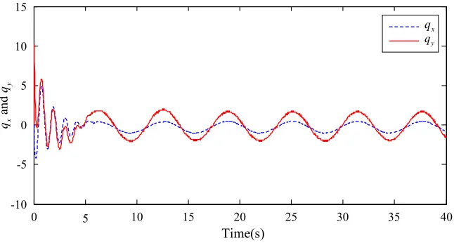
For the simulations, the initial state of the robot system is q=[ 0 −1.25 2 ]T. With the Assumption2, the final value of J∗ _is

chosen as 18.5470.

With the Lemma 2, design the parameters as follows:

1

1 0 0

0 0 0

0 0 0

n

 

 

=_{ }

 

 

, 2

1 0 0

0 0 0

0 0 0

n

 

 

=_{ }

 

 

and

1 0 0

0 1 0

0 0 1

T

 

 

Θ = Θ =_{ }

 

 

.

Here, design the cost function parameters as follows:

0.2545 0.3013 0.4589

0.1528 0.2354 0.0505

0.1466 0.2597 0.4267

c A

− − −

 

 

=_ − _

 ₋ 

 

,

1.448 0.4306

0.2577 0.0580

0.4313 3.1592

c B

 

 

=_ − _

_{− −} 

 

,

0.1246 0.3255 5.3794

0.74 0.5897 0.4890

0.1246 0.0946 0.2246

c C

− −

 

 

=_ − _

_{− −} 

 

Figure 1. The responses of system state variables q_x and q . _y

Figure 2. The response of system state variable q_θ .

Figure 3. The responses of system control inputs.

6. Conclusions

This paper addressed the dynamic output feedback control problem for a class of nonlinear system with multiple time-varying delay and parametric uncertainties. The nonlinear uncertainties are in the nonlinear form and bounded by nonlinear functions with gains unknown. The dynamic

compensator is designed and the control design condition is relaxed. The dynamic output feedback controller is constructed such that the solutions of the closed-loop system converge to an adjustable bounded region. The result is further extended to the general nonlinear case. Finally, the simulations for the mobile robot are performed and the results demonstrate the effectiveness of the proposed method.

0 5 10 15 20 25 30 35 40

-10 -5 0 5 10 15

Time(s)

y

q

x

q

an

d

x

y

q

q

Time(s)

0 5 10 15 20 25 30 35 40

-10 -8 -6 -4 -2 0 2 4 6 8 10

qθ

qθ

0 5 10 15 20 25 30 35 40

0 100 200 300 400 500 600 700

Time(s)

2 u

1 u

C

o

n

tr

o

l

in

p

u

Disclosure Statement

No potential conflict of interest was reported by the authors.

Funding

The authors wish to thank the editors and the anonymous reviewers for their valuable suggestions and critical comments to improve the paper. This research was financially supported by National Natural Science Foundation of China (Project No. 61473248); Natural Science Foundation of Hebei Province (Project No. F2016203496); National Intellectual Property Office of China (Grant No. ZL-2012-1-0052200.2; Zl-2012-1-0052199.3; Zl-2014-2-0411083.9); and China National Heavy Machinery research institute.

References

[1] M. Luo, C. S. Li, X. Y. Zhao, R. H. Li and X. L. An "Compound feature selection and parameter optimization of ELM for fault diagnosis of rolling element bearings." Isa Transactions 65 (2016): 556.

[2] C. S. Li, J. Z. Zhou, B. Fu. P. G. Kou and J. Xiao. "T–S Fuzzy Model Identification With a Gravitational Search-Based Hyperplane Clustering Algorithm." IEEE Transactions on Fuzzy Systems 20.2 (2012): 305-317.

[3] C. S. Li, J. Z. Zhou, P. G. Kou and J. Xiao. "A novel chaotic particle swarm optimization based fuzzy clustering algorithm." Neurocomputing 83.15 (2012): 98-109.

[4] C. C. Hua, Q. G. Wang, and X. P. Guan. "Adaptive fuzzy output-feedback controller design for nonlinear time-delay systems with unknown control direction." IEEE Transactions on Systems Man & Cybernetics Part B Cybernetics 39.2 (2005): 363-374.

[5] J. Wei, Y. Zhang, M. Sun, and B. Geng. "Adaptive iterative learning control of a class of nonlinear time-delay systems with unknown backlash-like hysteresis input and control direction." Isa Transactions (2017). DOI: 10.1016/j.isatra.2017.05.007. [6] L. Jing, and H. K. Khalil. "High-gain-predictor-based output

feedback control for time-delay nonlinear systems." Automatica 71 (2016): 324-333.

[7] O. M. Kwon, H. P. Ju, S. M. Lee, and E. J. Cha. "New augmented Lyapunov–Krasovskii functional approach to stability analysis of neural networks with time-varying delays." Nonlinear Dynamics 76.1 (2014): 221-236.

[8] I. V. Medvedeva, and A. P. Zhabko. "Synthesis of Razumikhin and Lyapunov–Krasovskii approaches to stability analysis of time-delay systems." Automatica 51 (2015): 372-377. [9] Éva Gyurkovics. "Guaranteed cost control of discrete-time

uncertain systems with both state and input delays." International Journal of Control 23.5 (2016): 1-13.

[10] Z. Wang, B. Shen, H. Shu, and G. Wei. "Quantized H-∞ control for nonlinear stochastic time-delay systems with missing measurements." IEEE Transactions on Automatic Control 57.6 (2012): 1431-1444.

[11] Q. Zhou, P. Shi. S. Xu, and H. Li. "Adaptive static output feedback control for nonlinear time-delay systems by fuzzy

approximation approach." IEEE Transactions on Fuzzy Systems 21.2 (2013): 301-313.

[12] F. Z. Gao, and Y. Q. Wu. "Global stabilisation for a class of more general high-order time-delay nonlinear systems by output feedback." International Journal of Control 88.8 (2015): 1540-1553.

[13] S. C. Tong, and Y. Li. "Adaptive fuzzy output feedback tracking back-stepping control of strict-feedback nonlinear systems with unknown dead zones." IEEE Transactions on Fuzzy Systems 20.1 (2012): 168-180.

[14] S. Y. Liu, Y. Liu, and N. Wang. "Nonlinear disturbance observer-based back-stepping finite-time sliding mode tracking control of underwater vehicles with system uncertainties and external disturbances." Nonlinear Dynamics (2016): 1-12. [15] Y. H. Choi, and S. J. Yoo. "Minimal-approximation-based

decentralized back-stepping control of interconnected time-delay systems." IEEE Transactions on Cybernetics (2016): 1-13.

[16] D. Huang, and S. K. Nguang. "State feedback control of uncertain networked control systems with random time delays." IEEE Transactions on Automatic Control 53.3 (2008): 829-834.

[17] Y. T. Wang, X. Lin, and X. Zhang. "State feedback stabilization for neutral-type neural networks with time-varying discrete and unbounded distributed delays." Journal of Control Science & Engineering 2012.1 (2012): 966-989.

[18] H. Q. Wang, P. X. Liu, and S. Peng. "Observer-based fuzzy adaptive output-feedback control of stochastic nonlinear multiple time-delay systems." IEEE Transactions on Cybernetics 99.5 (2017): 1-11.

[19] M. Wang, B. Chen, K. Liu, X. Liu, and S. Zhang. "Adaptive fuzzy tracking control of nonlinear time-delay systems with unknown virtual control coefficients." Information Sciences 178.22 (2015): 4326-4340.

[20] X. J. Xie, and L. Liu. "Further results on output feedback stabilization for stochastic high-order nonlinear systems with time-varying delay." Automatica 48.10 (2012): 2577-2586. [21] T. Dierks, and S. Jagannathan. "Neural network output

feedback control of robot formations." IEEE Transactions on Systems Man & Cybernetics Part B Cybernetics A Publication of the IEEE Systems Man & Cybernetics Society 40.2 (2016): 383-393.

[22] B. Ren, S. S. Ge, K. P. Tee, and T. H. Lee. "Adaptive neural control for output feedback nonlinear systems using a barrier Lyapunov function." IEEE Transactions on Neural Networks 21.8 (2015): 1339.

[23] J. Z. Peng, Y. Liu, and J. Wang. "Fuzzy adaptive output feedback control for robotic systems based on fuzzy adaptive observer." Nonlinear Dynamics 78.2 (2016): 789-801. [24] H. Yue, and J. Li. "Output-feedback adaptive fuzzy control for

a class of non-linear time-varying delay systems with unknown control directions." IET Control Theory & Applications 6.9 (2016): 1266-1280.

[26] Y. Li, and F. Gaob. "Optimal guaranteed cost control of discrete -time uncertain systems with both state and input delays." Journal of the Franklin Institute 338.1 (2016): 101-110. [27] M. S. Mahmoud. Resilient control of uncertain dynamical

systems. Springer, Berlin, Heidelberg, (2014).

[28] Y. He, G. P. Liu, D. Rees, and M. Wu. "Improved stabilisation

method for networked control systems." IET Control Theory & Applications 1.6 (2007): 1580-1585.