Extension of Numerical Matching Method to Weakly Nonlinear
Evolution of Resistive MHD Modes
Masaru FURUKAWA and Shinji TOKUDA
1)Graduate School of Engineering, Tottori University, Tottori-shi, Tottori 680-8552, Japan 1)Research Organization for Information Science and Technology, Shinagawa-ku, Tokyo 140-0001, Japan
(Received 14 March 2017/Accepted 1 May 2017)
We have extended “numerical matching method” to weakly nonlinear regime, which is relevant for the Rutherford regime of magnetic island evolution in normal magnetic shear plasmas as well as for reversed mag-netic shear plasmas to which the Rutherford theory does not apply. The numerical matching method was devel-oped for linear stability analyses of resistive magnetohydrodynamics (MHD) modes by utilizing an inner region with a finite width, that removes difficulties inherent in its numerical applications of the traditional matched asymptotic expansion. The extended method is applied to low-beta reduced MHD simulations of magnetic is-land evolution in cylindrical plasmas with normal and reversed magnetic shear profiles. The numerical results agree well with fully nonlinear simulation without using the matching method from the linear to weakly nonlinear regimes continuously. Since the nonlinear equation is solved only in the inner region of a finite width, the compu-tational cost is reduced, which enables us to include more detailed physics effects. Our extended method therefore makes a significant contribution in the MHD analysis of magnetic island evolution beyond the restriction in the conventional Rutherford theory.
c
2017 The Japan Society of Plasma Science and Nuclear Fusion Research
Keywords: magnetic island, nonlinear theory, matched solution using finite-width inner region, resistive magne-tohydrodynamics
DOI: 10.1585/pfr.12.1403025
1. Introduction
The theory of matched asymptotic expansion for lin-earized resistive magnetohydrodynamics (MHD) is well established [1]. After ten years of this pioneering work, the theory was extended to nonlinear regime [2]. Since then many applications of the Rutherford equation [2] have made much progress in fusion research, especially in the neoclassical tearing mode (NTM) studies [3–5]. Besides many numerical studies performed, the theoretical frame-work has been always based on the Rutherford equation essentially.
We have recently developed a new framework for the linear stability analyses of resistive MHD modes, i.e. the numerical matching method [6–8]. This method utilizes a finite-width inner region around a resonant surface, where the resistive MHD is solved, instead of an infinitely thin inner layer as in the traditional matched asymptotic expan-sion. The reason why we adopt a finite-width inner region is because it can remove difficulties inherent in numerical applications of the matched asymptotic expansion. For ex-ample, it is not easy to precisely compute the ratio of the diverging big to small solutions around the resonant sur-face numerically, which is required for the matched asymp-totic expansion, although sophisticated theories have been developed [9–12]. By using the inner region with a fi-nite width, we do not need to compute the ratio of the
author’s e-mail: [email protected]
big to small solutions for the matching. Instead, we need an appropriate boundary condition for the direct matching across the interfaces between the outer and inner regions. In [6], we developed such a boundary condition for the re-duced MHD [13, 14]. The important point is to impose a boundary condition such that the electric field along the magnetic field smoothly disappears as approaching from inner to outer regions. We developed both an eigenvalue and an initial-value approaches. In [7], another boundary condition was developed, which enables us to include in-ertia correction perturbatively to the outer solutions. Then the stability analysis of high beta plasmas has become pos-sible even if the plasma is close to its marginal stability. The diamagnetic drift effect was also taken into account by the inclusion of the inertia correction to the outer solu-tion [8].
In this paper, we extend the initial-value approach of the numerical matching method to weakly nonlinear regime. Namely, the nonlinear evolution equation is solved in the finite-width inner region, while the inertia-less lin-earized ideal MHD equation, or the Newcomb equation [15], is solved in the outer region. Then the solutions are matched at the interfaces between the outer and inner re-gions. This is the situation assumed in the Rutherford the-ory [2]. In Sec. 2, we firstly explain the setting of the prob-lem. The low-beta reduced MHD [13] is adopted for cylin-drical plasmas in this paper. We then develop the solution
c
2017 The Japan Society of Plasma
method for both the inner and outer regions as well as the matching condition. In Sec. 3, we show numerical results by the developed method. The first one is the Rutherford regime of magnetic island evolution in a normal magnetic shear plasma, while the second one is the nonlinear evolu-tion of double tearing mode in a reversed magnetic shear plasma. Both results agree well with fully nonlinear simu-lation without the matching method. In Sec. 4, we discuss four topics; namely, the importance of equilibrium com-ponents in the numerical results, the reduction of compu-tational cost, the significance of the application to the re-versed magnetic shear cases, and possible application to the high-beta toroidal plasmas. Then conclusions are given in Sec. 5.
2. Theory
2.1
Setting
In this study, we adopt the low-beta reduced MHD [13] in the cylindrical geometry as the simplest situation for demonstrating the principal ideas of our method. Let us consider a cylindrical plasma with minor radiusa and length 2πR0. The cylindrical coordinates are (r, θ,z). A toroidal angleζ:=z/R0is also used instead of the axial co-ordinatez. The inverse aspect ratio is given byε:=a/R0. Physical quantities are normalized by the length a, the magnetic field in thez-direction B0, the Alfvén velocity vA:=B0/
√μ
0ρ0withμ0andρ0being vacuum permeabil-ity and typical mass denspermeabil-ity, respectively, and the Alfvén timeτA:=a/vA. Then the low-beta reduced MHD equa-tions are
∂U
∂t =[U, ϕ]+[ψ,J]−ε ∂J
∂ζ, (1)
∂ψ
∂t =[ψ, ϕ]−ε ∂ϕ
∂ζ +ηJ. (2) Here, the fluid velocity is given byu = zˆ× ∇ϕ, and the magnetic field byB=zˆ+∇ψ׈z. The unit vector in thez direction is denoted as ˆz. The vorticity in thezdirection is U:=⊥ϕ, where⊥is the Laplacian in ther–θplane. The current density in thezdirection multiplied by a negative sign is given by J := ⊥ψ. The Poisson bracket for two functions f andgis defined by [f, g] :=zˆ· ∇f × ∇g. The inverse of the Lundquist number is denoted byη. Equa-tion (1) is the vorticity equaEqua-tion, and Eq. (2) is the parallel Ohm’s law.
Let us write the vector of the fields as u(x,t) := (ϕ(x,t), ψ(x,t))T, and let us assumeu = u
0(x)+u1(x,t) with u0 = (0, ψ0(r))T and u1 = (ϕ1(x,t), ψ1(x,t))T. Namely, the equilibrium is cylindrically symmetric, and has no plasma rotation. The time-dependent partu1is not necessarily small. Then the governing Eqs. (1) and (2) can be written in the following form:
M∂u1∂t =Lu1+N(u1), (3) where the explicit expressions for the the linear operators
MandL, and the nonlinear termN(u1) are
M= ⊥ 0 0 1 , (4) L= ⎛ ⎜⎜⎜⎜⎜ ⎜⎜⎜⎜⎜ ⎜⎝
0 ψ0,⊥ −[J0, ]−ε∂(∂ζ⊥ )
ψ
0, −ε ∂ ∂ζ η⊥ ⎞ ⎟⎟⎟⎟⎟ ⎟⎟⎟⎟⎟ ⎟⎠, (5) N(u1)= U1, ϕ1
+ψ
1,J1
ψ
1, ϕ1
. (6)
We set an inner region atrL <r < rR, which covers resonant surfaces of the mode under consideration. The outer region is the complement of the union of the in-ner region and the boundaries, given by 0 ≤ r < rL and rR < r < 1. Thus the interfaces arer = rRandr = rL. Extensions to multiple inner regions would be straightfor-ward.
2.2
Outer region
In the outer region, we solve the inertia-less, lin-earized ideal MHD equation or the Newcomb equation, which is given by the first row ofLu1 =0. Since the ge-ometry is cylindrical, we decompose the fields in a Fourier series as
u1=
m,n
umn(r,t)ei (mθ−nζ)
=
m,n
˜ ϕmn(r,t)
˜ ψmn(r,t)
ei (mθ−nζ), (7)
where mandn are poloidal and toroidal mode numbers, respectively. The Newcomb equation is given by
Nψ˜mn:=
1 r ∂ ∂r r∂ ∂r
−m
r
2
˜ ψmn+
mJ0(r) rk ψ˜mn
=0, (8)
whereNis the Newcomb operator and k(r) :=εm
1 q− n m . (9)
The prime denotes r derivative, and the safety factor is given byq(r) = −εr/ψ0(r). Equation (8) is the second-order, linear ordinary differential equation for ˜ψmn, and can
be solved independently for each pair ofmandn. The solu-tion can be expressed as a linear combinasolu-tion of two inde-pendent solutions. Let us construct the solution by Green’s functions defined by
NGψout,mn,p(r)=0,
Gψout,mn,p(rq)=δpq, p,q= L or R. (10)
Namely, the amplitude ofGψout,mn,p(r) is unity atr=rp, and
is imposed and thus one of the two independent solutions drops. At the plasma edge, we assume the fixed-boundary condition that also drops one of the two independent so-lutions. These are similarly imposed even if the magnetic axis or the plasma edge is in the inner regions. Now we express the outer solution as
˜
ψmn(r,t)=
p=L,R ˜
ψmn,p(t)Gψout,mn,p(r). (11)
We have included time dependence in the coefficients ˜
ψmn,p(t), which must be slow. From the outer region itself,
there is no way to determine ˜ψmn,p(t). It will be determined
through the matching condition with the inner solution in Sec. 2.4.
2.3
Inner region
In the inner region, we solve the nonlinear evolution Eq. (3). Let us discretize time with a constant intervalh, and denote the discrete time asti withi being an index.
Similarly, we writeui :=u(ti). If we adopt theKth-order
Adams–Moulton method (K=1,2,· · ·), an unknownui+1 is calculated by
Mui+1=Mui+h 1
k=2−K
ck
Lui+k+N(ui+k), (12)
wherecks are known constants. For example,c1 =1 for
K=1, which is the simplest implicit method as developed in [6]. It is extended to higher orders K ≥ 2 here. For K=2,c0 =c1 =12. The constants forK ≥3 are found in standard textbooks.
We rewrite Eq. (12) by moving the term linear inui+1 to the left-hand side and by separating out the nonlinear term ofui+1from the summation as
(M −c1hL)ui+1 =Mui
+h 0
k=2−K
ck
Lui+k+N(ui+k)+c1hN(ui+1). (13)
Then the last nonlinear term is unknown, while the remain-ings on the right-hand side are known. Thus we need an iteration for the last term to solve this equation. Therefore we introduce the following expression for the inner solu-tion
ui+ j J
mn(r)=
p=L,R ˜ ψi+Jj
mn,pGin,mn,p(r)+H i+Jj
in,mn(r),
j=0,1,· · ·,J, (14)
whereJis the maximum number of the iteration, and we assume thatui+
j J
mn(r) becomes sufficiently close tou i+j−J1 mn (r)
when j = J. The Green’s functions Gin,mn,p(r) =
(Gϕin,mn,p(r),Gψin,mn,p(r))Tis given by (M −c1hL)Gin,mn,p(r)=0,
Gψin,mn,p(rq)=δpq, p,q=L or R. (15)
The boundary condition for the ϕ component of the Green’s function, Gϕin,mn,p(r), was developed in [6], and is given such that the parallel electric field disappears smoothly as approaching from the inner to the outer re-gions. We need to calculate these Green’s functions only once at the beginning of the simulation becauseMandL do not change during the time evolution. Also the inho-mogeneous solution Hi+
j J
in,mn(r) = (H
ϕ,i+Jj
in,mn(r),H
ψ,i+Jj
in,mn(r))
T is obtained by solving
(M −c1hL)H
i+Jj
in,mn(r)=Mu i mn(r)
+h 0
k=2−K
ck
Luimn+k+Nmn(ui+k)
+c1hNmn(ui+
j−1
J ),
Hψ,i+ j J
in,mn(rp)=0, p=L and R, (16)
for j = 1,· · ·,J, where Nmn is the Fourier coefficient
of N(u). The boundary condition for Hϕ,i+ j J
in,mn is again the
smooth disappearance of parallel electric field, as same as the Green’s functions. The iteration must be performed to-gether with the determination of the amplitudes ˜ψi+
j J
mn,p
de-scribed in the next subsection.
2.4
Matching condition
In the numerical matching method, we impose conti-nuity ofψand its radial derivatives at the interfaces. First let us take ˜ψmn,p(t) in the outer region equal to ˜ψ
i+Jj
mn,q
appear-ing in the inner solution (14). Thenψbecomes continuous at the interfaces. Note thatpin the outer region andqin the inner region should be understood to express the same radial location. The remaining condition is the continuity of∂ψ/∂rat the interfaces, which is given by
p=L,R ˜ ψi+Jj
mn,p(Gψin,mn,p)(rq)+(H
ψ,i+Jj
in,mn)(rq)
=
p=L,R ˜ ψi+Jj
mn,p(G
ψ
out,mn,p)(rq), q=L or R, (17)
for each pair ofmandn. By solving Eq. (17), we obtain ˜
ψi+Jj
mn,p. Then we can evaluate the last term of Eq. (14) for
the next iteration.
3. Numerical Results
Here we show two kinds of simulation results of mag-netic island evolution. The first one is the Rutherford regime of magnetic island evolution in a normal magnetic shear plasma. The second one is the nonlinear evolution of the double tearing mode in a reversed magnetic shear plasma.
3.1
Normal magnetic shear plasma
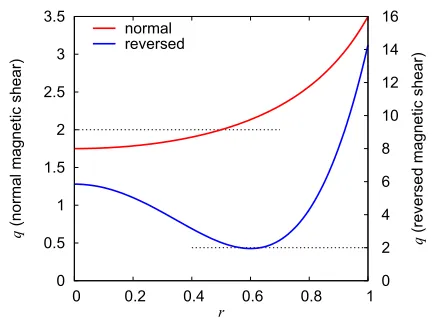
Fig. 1 qprofiles used in the numerical demonstrations.
q(r)= q0 1−r
2
2
, (18)
withq0 =1.75. Then theq =2 surface exists atr =0.5. Theq profile is shown as “normal” in Fig. 1. The other profile will be used in the next subsection. Them=2 and n=1 tearing mode is linearly unstable in this equilibrium; the tearing mode parameterΔm/n=2/1 22.4. The resistiv-ity was chosen to beη=10−6. Then the linear growth rate is 2.87×10⁻⁴ according to the corresponding eigenvalue problem.
In the present study, we only include Fourier com-ponents which are resonant at theq = 2 surface in the simulations, i.e., a mode family of m = 2 and n =
with =1,2,· · ·,L. The maximum numberLis chosen
to be sufficiently large so that the simulation result does not change much even whenL is further increased. For the results shown below, we took L = 5. The m = 0 andn = 0 components are not included in the numerical matching. Thus the equilibrium does not change during the simulation, which is similar to the situation of the Ruther-ford theory. We also performed fully nonlinear simulations without using the numerical matching for comparison. The m=0 andn =0 components are included for those sim-ulations. In the radial direction, we used the second-order finite difference method. The whole radial domain is di-vided into a hundred intervals with equal distance in this study. A mesh accumulation is of course possible in prin-ciple, or it would be better to do so, in order to increase the resolution inside the inner region. The time integration was performed by the first-order implicit method. The time interval wash=0.01.
Figure 2 shows the time evolution of (a) the kinetic energyEk and (b) the magnetic energy Em of them = 2 andn=1 component. Similarly, (c) and (d) show those of them=4 andn=2 component, and (e) and (f) them=6 andn = 3 component, respectively. Note that the linear eigenmode was used as the initial condition for m = 2 andn = 1, and that other components were taken to be
zero. In the figure, “num. match.” denotes our method, andΔr :=rR−rL denotes the width of the inner region. The q = 2 surface was taken to be at the center of the inner region, thusrL = 0.4 and rR = 0.6 for Δr = 0.2, andrL = 0.3, rR = 0.7 for Δr = 0.4. Also, “full” de-notes the result of the fully nonlinear simulation where the resistive reduced MHD equation was solved in the whole domain without the numerical matching. Especially, “full (m/n =0/0 unchanged)” means that them=0 andn=0 components were held unchanged during the fully nonlin-ear simulation. This situation is closer to the numerical matching. Also the linear growth is shown in Figs. 2 (a) and 2 (b) by the thin dashed lines. We observe that the en-ergy of them = 2 andn =1 mode grows linearly at the beginning (t0.3×104), which is followed by the weakly nonlinear or the Rutherford regime. We observe excellent agreement especially between the numerical matching re-sult withΔr=0.4 and the fully nonlinear simulation with m =n =0 mode kept unchanged even in the Rutherford regime; those curves are overlapping each other.
On the other hand, the results by the numerical match-ing, even withΔr =0.4, does not agree completely with the “full” result withm = n = 0 components being in-cluded. This indicates that the inclusion of them=n =0 components are crucial for achieving quantitative accu-racy. This requires further development of the theory.
We also observe that the numerical matching result withΔr =0.2 starts to deviate from the “full (m/n =0/0 unchanged)” result aroundt 104. Note that the simu-lation withΔr = 0.2 diverged after t > 1.5×10⁴. The deviation as well as the divergence are because the linear approximation in the outer region starts to break down as the perturbation grows. Indeed, the matching result with the wider inner regionΔr=0.4 agrees with the full simu-lation result for longer time.
Figure 3 shows the time evolution of the magnetic island width calculated by the amplitude of the m = 2 andn = 1 component of ψ. We again observe the ex-cellent agreement between the numerical matching result withΔr=0.4 and the full simulation result withm=n=0 mode kept unchanged. We also plotted a simulation result by solving the simplest Rutherford equation dw
dt =ηΔ
(w).
The initial island width was taken to be the same as that of the other simulations att =0.3×10⁴. It is not signifi-cantly different from our simulation results, except for the
Δr =0.2 case, although the degree of the agreement may depend on when we start the simulation of the Rutherford equation.
3.2
Reversed magnetic shear plasma
Fig. 2 Time evolution of kinetic and magnetic energy of several Fourier components in the normal magnetic shear plasma. “num. match.” denotes our matching method, “full” is the nonlinear simulation in the whole domain without the matching, and “(m/n =0/0 unchanged)” means that them=n=0 components are kept unchanged in the “full” nonlinear simulation. Fourier components of m=2andn=with=1,· · ·,5 are included in the simulation, while them=n=0 components are included only in “full”. For “num. match.”,Δrmeans the inner-region width. The matching results, especially withΔr=0.4, agree quite well with the full simulation withm=n=0 components kept unchanged for longer time. The linear approximation in the outer region starts to break down forΔr=0.2 att>∼104, leading to the deviation from “full”.
q(r)=qmin
⎡ ⎢⎢⎢⎢⎢
⎣(α−1)
r rmin
4
−2(α−1)
r rmin
2
+α
⎤ ⎥⎥⎥⎥⎥ ⎦,
(19) withqmin = 1.95, rmin = 0.6 and α = 3. Theq profile is plotted as “reversed” in Fig. 1. There exist twoq = 2
ra-Fig. 3 Time evolution of the magnetic island width. The keys are the same as in Fig. 2. The island width is calcu-lated from the amplitude of them/n = 2/1 component ofψ. Furthermore, numerical solution of the Rutherford equation is also plotted. After the initial linear growth (t0.3×104), the time evolution enters the Rutherford
regime. We observe the good agreement as in the time evolution of energy in Fig. 2.
dial grids; We took two hundred grids with equal spacings in the whole minor radius of the plasma.
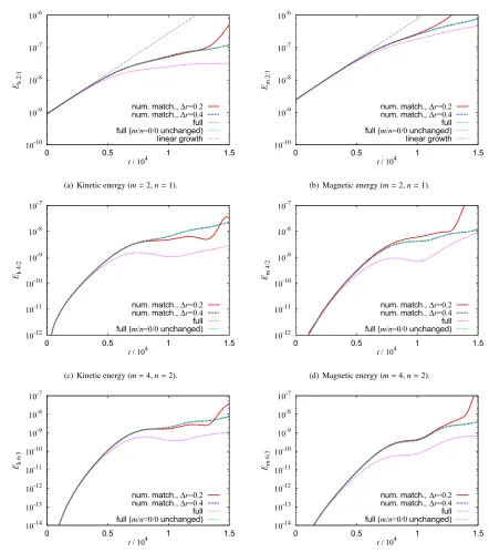
Figure 4 shows the time evolution of (a) the kinetic energyEk and (b) the magnetic energy Em of them = 2 andn = 1 component, (c) and (d) those of the m = 4 andn =2 component, and (e) and (f) those of them =6 andn = 3 component, respectively. Because theq = 2 surfaces exist near theqminsurface atr=0.6, we took the inner region asrL = 0.5 andrR = 0.7 forΔr = 0.2, and rL = 0.4, rR = 0.8 for Δr = 0.4. We observe the good agreement especially between the result of the numerical matching withΔr =0.4 and the full simulation withm = n = 0 components kept unchanged. The simulation by the numerical matching method withΔr = 0.2 diverged because of the same reason as in Fig. 2.
4. Discussion
In this section, let us discuss four topics. The first one is the difference concerning them=n=0 components be-tween the normal and reversed magnetic shear cases shown in the previous section. The second one is the reduction of the computational cost. The third one is the significance of the application to the reversed magnetic shear case, and the last one is the possible application to the high-beta toroidal plasmas.
4.1
Di
ff
erence of
m
=
n
=
0
components
In this subsection, we discuss the difference concern-ing them=n=0 components between the normal and re-versed magnetic shear cases. Comparing these two cases, the deviation from the “full” result, includingm =n = 0 components, may be larger in the reversed magnetic shear case in Fig. 4 than in the normal magnetic shear case in
Fig. 2. This is because the energy of them=n =0 com-ponents is dominant in the reversed magnetic shear case, while it is sub-dominant in the normal magnetic shear case. Figure 5 shows the radial profiles of the real parts of the m/n=0/0 and 2/1 components ofψobtained by the fully nonlinear simulation. The imaginary parts are zero. Fig-ures 5 (a) and 5 (b) are the normal and the reversed mag-netic shear cases, respectively.
For the normal magnetic shear case in Fig. 5 (a),t = 5000 and 15000 are selected as typical timings. The time evolution at t = 5000 is the beginning of the nonlinear phase, andt = 15000 is much later. As we observe, the m=n=0 component is smaller than them=2 andn=1 component at both timings. The energy of them=n=0 components is thus sub-dominant. Because the equilib-riumm=n=0 component does not change significantly, the magnetic islands do not saturate even att=15000.
On the other hand, for the reversed magnetic shear case shown in Fig. 5 (b), we observe that them = n = 0 component is considerably larger than them=2 andn=1 component at t = 3500 which is in the fully nonlinear phase. In the beginning of the nonlinear phase,t =1500, them= n =0 component is smaller than them= 2 and n = 1 component. Thus the energy of the m = n = 0 components is dominant at t = 3500, which causes the quasi-linear saturation of the double tearing mode in the fully nonlinear phase.
Interestingly, them=n=0 component is finite within the inner region withΔr = 0.4 in the reversed magnetic shear case, while it is almost zero in the outer region. Be-cause them = n =0 component is large in the inner re-gion, the deviation between the numerical results with and without them =n =0 component is large. However, be-cause them= n = 0 component is localized in the inner region withΔr =0.4, the quantitative accuracy can be re-covered if them=n=0 component is also solved only in the inner region of the numerical matching. The Dirichlet boundary condition may be appropriate for them=n =0 component. For the normal magnetic shear case, on the other hand, them=n=0 component extends to the outer region, especially at the smallerrregion. Because the am-plitude of them = n = 0 component is not so large, the deviation between the numerical results with and without them = n = 0 component is smaller. However, we may need to match them=n=0 component at the interfaces between the outer and the inner regions for this case. The matching of them = n = 0 components requires further development of the theory, which is our future issue.
4.2
Reduction of computational cost
match-Fig. 4 Time evolution of kinetic and magnetic energy of several Fourier components in the reversed magnetic shear plasma. The keys are the same as in Fig. 2. We observe quite good agreement between the numerical matching result withΔr =0.4 and the full simulation withm=n=0 components kept unchanged. The simulation withΔr=0.2 diverged because of the same reason as in the normal magnetic shear case, i.e., the breakdown of the linear approximation of the outer solution.
ing solutions, while we used the second-order Runge-Kutta method for the full simulation. For this point, we ex-pect that the computational time will not change much for the matching solution even if the second-order algorithm is used, because the formulation is given by the Adams method where the past data required for the next step are stored. Then the computational time for the matching so-lution withΔr=0.2 was about 1/3 of the full simulation
Fig. 5 Radial profiles of the real part ofψform/n=0/0 and 2/1 components obtained by the fully nonlinear simulations. (a) and (b) are the normal and the reversed magnetic shear cases, respectively.
4.3
Significance of application to reversed
magnetic shear plasmas
Let us here emphasize that our matching method ap-plies even if the magnetic shear vanishes at theqmin sur-face, e.g. qmin = 2 for them = 2 andn = 1 mode. The Rutherford theory does not apply to this situation from the beginning. On the other hand, such aqprofile can be im-portant in advanced operations. In our previous paper, we have proven that our method calculates the linear stability of this particular situation correctly with no difficulty [6]. Another interesting situation is that the two resonant sur-faces are well separated in radius. Then two separated in-ner regions should be appropriate. Theoretically no diffi -culty will arise since we only need to match the resonant poloidal Fourier components. This may be different from the case with multiple inner regions in toroidal plasmas, which we will discuss in the next subsection.
4.4
Application to high-beta toroidal
plas-mas
In this subsection, we discuss application of our matching method to high-beta toroidal plasmas. We have already proven that the numerical matching method can correctly handle the internal kink mode in a cylindrical plasma that simulates the high-beta toroidal plasmas close to the marginal stability [7] because the tearing mode pa-rameter Δ diverges positively [16] as the internal kink mode. In toroidal plasmas, we need to construct numer-ically matched solutions using multiple inner regions. Al-though a prototype of this kind of code has been developed for the linear stability [17], where non-resonant poloidal Fourier components were also matched, the boundary con-dition for the non-resonant components seems to be more improved.
5. Conclusions
We have extended the numerical matching method to weakly nonlinear cases, which is relevant for the Ruther-ford regime of magnetic island evolution in normal mag-netic shear plasmas as well as for the reversed magmag-netic shear plasmas to which the Rutherford theory does not ap-ply. We presented two demonstrations of the numerical matching method. One is the Rutherford regime of mag-netic island evolution in a normal magmag-netic shear plasma, while the other is the nonlinear evolution of double tearing mode in a reversed magnetic shear plasma. We observed excellent agreement between the numerical matching re-sults and the fully nonlinear simulations withm =n =0 components kept unchanged. On the other hand we recog-nized the importance of them=n=0 components for the quantitative accuracy. The quasi-linear saturation of the double tearing mode in the reversed magnetic shear case may be simulated accurately if them=n=0 components are solved only in the inner region, because that compo-nent is localized in the inner region. Generally, however, we need further development of the theory for including the change of them=n=0 components for the quantita-tive accuracy.
asymp-totic expansion in a deeper theoretical context, our method will aid understanding physics of MHD activities such as NTMs, and will bring about qualitative changes in MHD analysis of fusion plasmas.
Acknowledgments
This work was supported by KAKENHI Grant No. 23760805 and No. 15K06647.
[1] H.P. Furth, J. Killeen and M.N. Rosenbluth, Phys. Fluids6, 459 (1963).
[2] P.H. Rutherford, Phys. Fluids16, 1903 (1973).
[3] A.I. Smolyakov, Plasma Phys. Control. Fusion 35, 657 (1993).
[4] O. Sauter, R.J. La Haye, Z. Changet al., Phys. Plasmas4, 1654 (1997).
[5] R.J. La Haye, Phys. Plasmas13, 055501 (2006).
[6] M. Furukawa, S. Tokuda and L.-J. Zheng, Phys. Plasmas
17, 052502 (2010).
[7] M. Furukawa and S. Tokuda, Phys. Plasmas18, 062502 (2011).
[8] M. Furukawa and S. Tokuda, Phys. Plasmas19, 102511 (2012).
[9] A. Pletzer and R.L. Dewar, J. Plasma Phys.45, 427 (1991). [10] A. Pletzer, A. Bondeson and R.L. Dewar, J. Comput. Phys.
115, 530 (1994).
[11] S. Tokuda and T. Watanabe, J. Plasma Fusion Res.73, 1141 (1997).
[12] S. Tokuda, Nucl. Fusion41, 1037 (2001). [13] H.R. Strauss, Phys. Fluids19, 134 (1976). [14] H.R. Strauss, Phys. Fluids20, 1354 (1977). [15] W.A. Newcomb, Ann. Phys.10, 232 (1960).
[16] D.P. Brennan, E.J. Strait, A.D. Turnbull, M.S. Chu, R.J. La Haye, T.C. Luce, T.S. Taylor, S. Kruger and A. Pletzer, Phys. Plasmas9, 2998 (2002).