Online Feature Selection (OFS)
with Accelerated Bat Algorithm (ABA)
and Ensemble Incremental Deep Multiple Layer
Perceptron (EIDMLP) for big data streams
D. Renuka Devi
*and S. Sasikala
Abstract
Feature selection is mainly used to lessen the dispensation load of data mining models. To condense the time for processing voluminous data, parallel processing is car-ried out with MapReduce (MR) technique. However with the existing algorithms, the performance of the classifiers needs substantial improvement. MR method, which is recommended in this research work, will perform feature selection in parallel which progresses the performance. To enhance the efficacy of the classifier, this research work proposes an innovative Online Feature Selection (OFS)–Accelerated Bat Algo-rithm (ABA) and a framework for applications that streams the features in advance with indefinite knowledge of the feature space. The concrete OFS-ABA method is suggested to select significant and non-superfluous feature with MapReduce (MR) framework. Finally, Ensemble Incremental Deep Multiple Layer Perceptron (EIDMLP) classifier is applied to classify the dataset samples. The outputs of homogeneous IDMLP classifiers were combined using the EIDMPL classifier. The projected feature selection method along with the classifier is evaluated expansively on three datasets of high dimension-ality. In this research work, MR-OFS-ABA method has shown enhanced performance than the existing feature selection methods namely PSO, APSO and ASAMO (Acceler-ated Simul(Acceler-ated Annealing and Mutation Operator). The result of the EIDMLP classifier is compared with other existing classifiers such as Naïve Bayes (NB), Hoeffding tree (HT), and Fuzzy Minimal Consistent Class Subset Coverage (FMCCSC)-KNN (K Nearest Neigh-bour). The methodology is applied to three datasets and results were compared with four classifiers and three state-of-the-art feature selection algorithms. The outcome of this research work has shown enhanced performance in accuracy and less processing time.
Keywords: Feature selection, Online Feature Selection (OFS), Big data, Ensemble Incremental Deep Multiple Layer Perceptron (EIDMLP), Accelerated Bat Algorithm (ABA), MapReduce (MR)
Open Access
© The Author(s) 2019. This article is distributed under the terms of the Creative Commons Attribution 4.0 International License
(http://creat iveco mmons .org/licen ses/by/4.0/), which permits unrestricted use, distribution, and reproduction in any medium,
provided you give appropriate credit to the original author(s) and the source, provide a link to the Creative Commons license, and indicate if changes were made.
RESEARCH
*Correspondence: renukadevi.research@gmail. com
Introduction
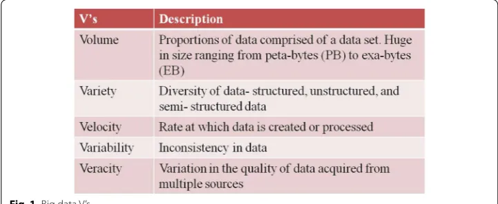
Big data refers to any assortment of data which are outsized and intricate in nature such that conventional database administration systems and data processing tools cannot process. Big data can be characterized by 5 V’s [1, 2] namely “Volume”, “Variety”, “Veloc-ity”, “Variabil“Veloc-ity”, and “Veracity” (Fig. 1).
From the perception of these challenges, it is acknowledged that the conventional data mining methods are neither appropriate for data stream of diverse characteristics nor to achieve the analytical efficiency as it involves periodic analytics in contrast to big data which involves real-time analytics. Also, every time the induction model has to re-run and rebuilt for adding up of the recent data. Besides, to ensure scalability, MapReduce framework [3–5] is implemented to parallelize the classification algorithm. Presently, many Machine Learning (ML) techniques are premeditated to big data analytics [6]. For glitches involving big data sets of varied type and nature, deep learning (DL) techniques were formulated for improved performance classification.
DL algorithms are quite beneficial as it handles multifaceted, complex and unstruc-tured data by a greedy layer-wise learning [7, 8]. DL procedures have provided signifi-cant contributions along with ML applications explicitly speech recognition systems [9], computer vision [10], and NLP [11]. DL has been proficiently used for addressing viva-cious issues in big data analytics.
Feature selection (FS) is a momentous step in any classification application. It becomes a complex task when data features are huge. For several years, many research works have focused on FS methods [12, 13]. FS essentially involves the removal of extraneous and redundant features, thereby creating a prediction model with higher efficiency, inter-pretability, and speed. FS has been applied to many applications involving high dimen-sional data. Though, comprehensive methods are accessible for FS, there is an exposed challenge in handling rapid big data streams that requires instantaneous processing.
The current literature features many FS methods, but they are conducted in batch mode rather online. In offline mode, all features are available for training before the FS process. Taking into consideration of real-time applications, features may arrive online and accumulation of all training examples becomes expensive. So, OFS [14] is intro-duced for selecting the features using an online learning approach. In order to extract significant perceptions from big data sets in the online learning process, several relevant
features must be efficiently identified. These features have to be also effectively identified from the big data sets so that accurate prediction models can be built in real time. The OFS with data streams is closely associated with data stream mining [15].
When data becomes uncontrollable or huge, the parallel processing is employed for reducing the time complexity. In this research effort, an ascendable efficient OFS method using the parallel Accelerated Bat Algorithm (ABA) technique is proposed to select the features from the data set online. In addition, the proposed Ensemble Incremental Deep Multiple Layer Perceptron (EIDMLP) classifier is used for large scale data. To work with large-scale dataset, a distributed programming model, MapReduce is used which divides the dataset into smaller portions. The scalability of OFS-ABA over an extremely high dimensional and big dataset is proven through an empirical study which also demon-strates, that the algorithm performs superlatively well than the other state-of- the-art FS methods.
This research work is structured into various segments. The segment on “Literature review” skeletons the related work done in the field of feature selection and classi-fication, and the motivation behind this research work. The “Proposed methodology” section describes the proposed method in a step by step process, starting from pre-pro-cessing to classification. The “Experimental work” section mandates the datasets used, the evaluation metrics, and the outcomes are envisaged as tables and diagrams. The final section, “Conclusion” recapitulates the entire work.
Literature review
Feature selection (FS) technique for big data analytics is envisioned to have a significant feature selection method with reduced time complexity and enhanced accuracy levels. The recent progresses in OFS with MapReduce have given a major revolution in this domain. In the recent years of development, bio-inspired associated algorithms have been used for various problems of big data analytics [16].
Hoi et al. [14] has architected an effective algorithm that provides a solution to the problem by giving a theoretical analysis and assessing the performance empirically for OFS on benchmark datasets. The application of OFS was established on real time issues, which significantly scales when compared to other FS algorithms. The outcomes are vali-dated with the efficacy of the projected techniques for extensive and varied large scale applications.
Peralta et al. [17] projected a MapReduce approach to derive a subset of features from large data sets. The FS method was assessed by classifiers such as support vector machine (SVM), Naïve Bayes (NBs) along with logistic regression (LR). The evaluations showed that the spark implemented framework was beneficial to perform evolutionary FS on large data sets with enhanced classification precision and runtime. Tsamardinos et al. [18] accessed the Parallel, forward–backward with pruning (PFBP) algorithm for FS for huge datasets. The experimental study demonstrated increased scalability (num-ber of features) with speedup.
base kernel is associated with a set of features. The results show an improved training, competence over bigger data with ultra-large sample size.
De la Iglesia et al. [20] swotted diverse Evolutionary Computation (EC) for FS in clas-sification problems. The development of EC is the competence to efficiently search large population. The assessment and implementation uncovered the competency of these algorithms and further leads to new research direction in FS problems. Nazar and Sen-thilkumar [21] contributed an efficient, scalable OFS, which used the Sparse Gradient (SGr) for the online selection of features. In this approach, based on the threshold value, the feature weights were proportionally decremented, which zeroed irrelevant featured weights. The experimental results demonstrated heightened accuracy of 15% compared to other methods.
Hu et al. [22] elaborated on a conventional online FS stream dataset. A comprehensive review of the present OFS method was analyzed and compared over other methods. The uncluttered issues were discussed in FS. Yu et al. [23] built a Scalable and Precise Online Feature Selection (SAOLA), online FS model built on pair wise comparison techniques and extended to online group FS. On the augmentation side, SAOLA algorithms were scalable, on high dimensional data sets. It exhibited a superior performance compared to other prevailing algorithms.
The review of the feature selection methods for handling data stream has been dis-cussed in many recent works [24–29]. Fong et al. [24] proposed a novel, lightweight Accelerated Particle Swarm Optimization (APSO) feature selection algorithm for big data streams. The APSO algorithm is based on swarm intelligence and the proven results show that the algorithm performed well in terms of accuracy, time complexity, and so on. Five benchmarks datasets are experimented in this work.
Said and Alimi [25] crafted a Multi-Objective Automated Negotiation based Online Feature Selection (MOANOFS). The results demonstrated that MOANOFS system can be successfully applied to diverse domains and were able to accomplish high accuracy on real time applications. Lin et al. [26] estimated an improved cat swarm optimization (ICSO) algorithm for big data classification. The algorithm is pragmatic for FS in text classification problems in big data analytics. The proposed ICSO is compared with CSO. The disadvantage here is, it was only pertinent to text classification problems.
Gu et al. [27] projected the competitive swarm optimizer which is a variant of the PSO algorithm, overcomes the shortcomings of conventional PSO when handling large scale datasets, with less computational cost. The algorithm performs FS to select minimal sub-sets followed by classification. The future work is protracted to explore multi-objective, meta-heuristics FS algorithm to handle huge dimensionality with enhanced accuracy.
Manoj et al. [28] prospectively came up with the ACO–ANN algorithm for FS in big data analytics for text classification. The challenge in terms of this approach is to apply other types of data such as images and video. The exertion emphasized the use of pop-ulation-based hybrid algorithm for FS problems. Devi et al. [29] proposed the Multi-Objective Firefly and Simulated Annealing for online feature selection where the KSVM classifier was used for classification. This scheme had the limitation of having only one classifier and the performance was not compared with the other classifiers.
behaviour analysis. The proposed classifier has demonstrated enhanced performance in terms of accuracy compared with other algorithms. Young et al. [31] outlined the DL based ensemble approach for prediction in big data analytics. This work highlighted the issues of conventional mining, and proved the elevated performance level of Deep neu-ral networks.
From the prevailing literature, it can be deduced that the bio-inspired algorithm com-bined with the MapReduce approach evidences to be effectual and competent in Feature selection (FS) methods in the field of big data analytics. It is evident that DMLP is used for classification problems.
Proposed methodology
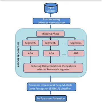
MapReduce model is applied to big datasets, which is further divided into smaller par-tition. In the proposed, an efficient scalable Online Feature Selection (OFS) approach using the Accelerated Bat Algorithm (ABA) technique was recommended for OFS. In this approach, based on the threshold values, the feature weights are proportionally dec-remented and Clustering Coefficients of Variation (CCV) zeroed incognizant features weights. This work suggested an Ensemble Incremental Deep Multiple Layer Perceptron (EIDMLP) classifier for large scale data. Also, we have analyzed the impact with a pen-alty and kernel parameters on the performance of EIDMLP classifier. The scalability of OFS- ABA over an extremely high dimensional and big dataset is proven through an empirical study which also illustrates that the algorithm performs supremely improved than the other known FS methods. The proposed model is shown in Fig. 2.
Preprocessing
Normalization is commonly used to maintain the balance of significance amongst the attributes, when attributes are on a diverse scale. When datasets are with diverse range of attributes, they are preprocessed by min–max normalization method. In this process all the values are transferred into same scale between 0 and 1, thus giving importance to the attribute even with the low range of value on scale.
It is the method of scaling the given dataset within the specified range of values between 0 and 1. From the Eq. (1), the normalized feature is derived.
where n is the current value of the feature and n’ is the normalized value of the fea-ture. minds is the minimum value and maxds is the maximum value of the given dataset. nfmax and nfmin is the normalization range 0, 1 respectively.
OFS
OFS [14] is related to streaming features. The interpretation of OFS [21] is represented by the notation Ds = [Ds1, Ds2,…,Dsn]T∈ Rn×d, Where Ds1,…,Dsn is the given dataset with the feature set Fs = [fs1, fs2,…, fsd]T∈ Rd and let Cl = [cl1, cl2,…,clm]T∈ Rm denote the class label vector. Let d be the number of features which is unknown in priori, the best (1)
n′= n−minds maxds-minds
feature subsets are selected from d such that s < d. Accuracy will be achieved through only selecting the most relevant feature subset for classification. For every Dsi, feature weight vector wei∈Rd is learned which classifies the instance. After classification, wen is updated to wen+1 . For features of streaming nature, the number of features is unknown priori, consequently this issue is well handled by OFS. The OFS acquire dataset instance one at a time. For every instance, a weight vector is learned and the class label of the instance is prophesied using the function sign (wen′×Dsn) . Followed by, comparison of
target and predicted class is done. The weight vector is rationalized using the following stochastic gradient rule given in Eq. (2) when the method misclassifies:
In Eq. (2), C′
wen,Dsn,yn implies the cost function and α denotes the rate of the learning. This procedure is concisely specified by EIDMLP classifier.
(2)
wen+1=wen−αC′�wen,Dsn�,yn
MapReduce
In MapReduce model, the given dataset (Ds) is spilt into number of smaller sets and
distributed across the network [32] and for every single partition the feature selection algorithm is applied in parallel. The examples are equally distributed and processed in parallel so as to achieve the class balance. In MR, (Dsi) is mapped into the corresponding
mapi task. Throughout the mapping phase, Dsi comprises of the OFS (in this case, based
on ABA).
ABA is applied to each partitions, the output of each map function is represented as fei =fei1,. . .,feiD , where the number of selected features is denoted by ‘D’. The reduce phase combines the features selected from each partitions, obtaining a vector ‘sf’ given in Eq. (3), where sfj denotes the jth feature.
This is the outcome of the complete OFS process, which is used for further ML process:
where n = number of tasks in the MapReduce. Generally the reduce phase is carried out by a distinct process thus reducing the execution time in MR [33]. The entire execution is done with a single MR process which eliminated the added disk admittances.
Accelerated Bat Algorithm (ABA)
The Accelerated Bat Algorithm (ABA) is formed on the echolocation activities of bats. Bats collect the information of the streaming features. Microbats are capable of echolo-cation, a fascinating characteristic they possess to find optimal streaming features and classify. The process is given as follows [34, 35]:
1. Bats discover food and prey using echolocation.
2. Every bat has velocity vei, with a feature position fpi with freqmin fixed frequency,
varying wavelength and A0 loudness. The pulse emission rate varies between
er∈[0, 1] . The wavelength is modified accordingly.
3. The loudness is from A0 to Amin.
freq take the values in a range [freqmin, freqmax] that correlate to wavelengths
[min,max ]. At time step t, outline the rules how feature position fp
i and velocities vei in a higher dimensional population is given by the following Eqs. (4) to (6) [36].
where β∈[0, 1] is a random vector drawn from a uniform distribution.
(3)
sf =
sf1,. . .,sfD, sfj=
1 n
n
i=1 feij
(4)
freqi =freqmin+freqmax−freqminβ
(5) veti =veit−1+
fpti−fp∗ freqi
Here fp∗ is the current global best solution which is updated on every iteration in comparison with the current position for ‘n’ number of features with the velocity ifreqi .
The best feature is selected amongst the current best optimal feature using random walk
where ǫ∈ [− 1, 1] is a random number with a loudness average At=
Ati
. Both Ai and
eri of pulse emission rate is adapted consequently. The loudness and pulse emission rates
are contrariwise proportional. To set the starting position for applying ABA, some fea-ture ranker function and mutation operator is applied to augment the accuracy of the classifier. Initial position of the BA is rearranged by using the Gaussian Mutation opera-tor. Let fi∈[ai,bi] be a real variable. Then the truncated Gaussian mutation operator
changes fi to a neighboring value using the following probability distribution [37]:
where ϕ(z)= √1
2πexp
−12z2
is the probability distribution of the standard normal dis-tribution and Φ(·) is the cumulative distribution function.
This mutation operator has a mutation strength parameter σi for every features, which should be related to the bounds ai and bi, σ =σi/(bi−ai) as a fixed non-dimensionalized parameter for all m features. To implement the above concept use the following Eq. (9 to 11) to compute the offspring f′
i:
where α = 38π ((π−3)
4−π )≈ 0.140012 and sign
u′i
is − 1 if u′i < 0 and is + 1 if u′i ≥ 0. Also, uL
and uR are calculated as follows
Thus, the Gaussian mutation procedure for mutating i-th feature variable fi is as follows:
(7) fpnew=fpold+ǫAt
(8)
p�
fi′,fi,σi�= 1 σiφ
� fi′−fi
σi �
φ�bi−fiσ
i �
−φ�ai−fiσ
i
� if ai≤fi′≤b
0 otherwise
(9) fi′=fi+√2σ (bi−ai)erf−1
u′i
(10) u′i=
2uL(1−2ui), if ui≤0.5
2uR(2ui−1), otherwise
(11) erf−1�
u′
i
� ≈sign�
u′ i � � � � � � 2 π α+ ln� 1−u′i2�
2 �2
−ln �
1−u′i2� 2 −
� 2 π α+
ln� 1−u′i2�
2 � 1/2 (12) uL=0.5
erf
a
i−fi
√
2(bi−ai)σ
+1
(13) uR=0.5
erf
b
i−fi √
2(bi−ai)σ
+1
Step 1: Create a random number ui∈ [0, 1]. Step 2: Use Eq. (9) to create offspring f′
i from parent fi
CCV is used as fitness function [38] to select the optimal features with a balance between class and overfitting problem. This function is mainly applied for building an accurate prediction model. Higher the CV, the features are considered.
Let Ds be a dataset with n instances and m features. An instance
f1,f2,. . .,am is
divided into number of groups with classes c∈C is the total number of prediction target
classes. For each fa,a∈[1..m] , fa∈fa1,fa2,. . .,fac
vd is the sum of all coefficients of variation for each class c where c∈[1..C] , for that par-ticular ath feature.
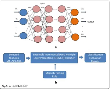
Ensemble Incremental Deep Multiple Layer Perceptron (EIDMLP)
The Deep Multiple Layer Perceptron (DMLP) is experimented to improve classifica-tion results of big data stream. An ensemble method combines the output of individual homogenous classifiers applied to the given big datasets. Output from each ensemble is selected and combined using majority voting rule [39]. DMLP is a multiple feed forward artificial neural network that maps input vectors to that of the output vectors. It is a (14)
vd=
c
c=1
n n=1
fc n−fac
2
n
fc a
connected graph with numerous layers namely input, hidden, and output layer. In this fully connected network, one to one layer connectivity is established. Also, it allows one or more hidden layers. Except for input layer nodes, rest of other neurons are associated with a nonlinear activation function. DMLP, an leeway of a single-layer perceptron cor-rects the weakness that single layer perceptron that cannot unravel nonlinear data with 3 ensembles. It can learn separable decisions non- linearly. It is shown in the Fig. 3.
In DMLP [30], five or ten hidden layers are implemented in contrast to the conven-tional simple two layer MLP. Generally, sigmoid and tanh activation functions show elevated performance in small to medium sized networks. By hard preventive the input of undesirable hidden nodes to zero, the function permits them to obtain sparse depic-tions. The term shortcut is the connection that span across the multiple layers. But, in DMLPs shortcuts are generally avoided hence all nodes of one layer is connected with the subsequent layer.
The following are the list of nodes(j) in the layers:
• Succ(i) is where is connection i → j exits.
• Pre(i) is where is a connection j → i exits.
For every connection between the layer i and layer j, the weight weji is assigned. All hidden and productivity nodes have a network input neti and aci activation output. In mining streaming data, data instances are generated frequently over the time. The issue arises to update the model every time without reloading the entire batch. This frequent updation even becomes very crucial if the data examples are massive. The model should be updated incrementally. To solve this incremental problem, an incremental DMLP classification model is proposed. The method is also named any-time algorithm as big dataset samples are read only once without the need to store or reload the samples every time. A tree is built by the induction method which selects an attribute to be classified by estimating the necessary indicators that registers the counts of every attribute value. To compute the frequency of attribute value atij of attribute ati corresponding to class yk, the Hoeffding Bound (HB) [38] is calculated using Eq (15).
where R is the class distribution and n is the number of instances that are perceived to a class. At any particular time, the top value of H(.) called atia= argmax (atia).
Similarly, the second top value is atib, where atib=argmax H (atij),∀≠. The two top values are incrementally taken as induction leaves and new data comes. The value ΔH
(ati) = Δ H (atia) − Δ H (atib) is calculated for each attribute atib where i ∈ I as the differ-ence between the two calculated top values. Using Eq. (16), a confidence interval is com-puted as rtrue, for the n number of instances till then. This is done to confirm the relation of attribute value atij to class yk. The confidence intervals are observed incrementally as the only statistics for each attribute ATi, r−HB≤ rtrue< r+HB where=(1/)Σri is retained. When the equality and rtrue < 1 hold true over the observed samples, then the tested ati ,
(15)
HB=
R
2ln1
δ
is the best statistical candidate with good accuracy among part of the data stream in entirety.
The classified outputs of IDMLP classifier is now combined using Majority Voting. Let Tri be total set of examples (N) and CL be a set of output (Q) classes. Let S = {A1, A2, AM} be an algorithm set which contains the M classifiers to be used for voting. Every example
TR ∈ri , the prediction is made and the Classifier Q has all the predicted classes. Here,
final class assigned is the class of each example predicted by the majority of classifiers by gaining majority votes which is explained as follows. Let cll∈CL denotes the class of an example ‘tr’ predicted by a classifier Al, and let a counting function Fk defined as:
where cll and clk are the classes of CL. The sum of entire votes for class clk and it is
defined via the use of the major vote function ( mvMk):
S is the set of class that gained the majority of vote, with class cl for example tr is given as:
Two strategies are used when more than one class conflicts with the same vote. The classes are arbitrarily chosen (SMV) in the first strategy whereas in the second strat-egy, an Influence Majority Vote (IMV) chooses the class given by the ensemble’s best classifier.
(16)
Fk(cll)=
1 cll =clk
0 cll�=clk
(17)
mvMk=Tck =
M
l=1 Fk(cll)
Experimental work
Dataset
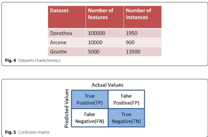
The proposed methodology is implemented with benchmark mark dataset from the “UCI repository”. The characteristics of big datasets experimented is shown in the Fig. 4. Arcene dataset consists of 10,000 features and 900 instances. This dataset was merged from the mass spectrometry datasets. Based on the numerous feature characteristics, the cancer patient has to be identified from the healthier one from the dataset.
The Dorothea dataset consists of various molecular properties of drug combination. The molecular features must be either active or inactive combination for drug formation. The classification task is to identify the molecules of binding nature or not. The identifi-cation of the binding property further leads to designing the new drug compounds with added properties like absorption, duration of action etc.,
The gisette dataset is used for hand written digit recognition, has 13,500 instances and 5000 features. The challenge here is to classify the digits four and nine. The distractive features were added into the dataset for feature selection.
Performance evaluation
The performance results are measured in expressions of Accuracy, Precision, Recall, F-measure, Processing time.
Sensitivity is also known as the true positive rate (TPR) which evaluates the amount of positives that are appropriately identified as positive.
From the confusion matrix (Fig. 5), precision is interpreted as follows:
(19)
TPR=Recall= TP
P =
TP (TP+FN)
Fig. 4 Datasets characteristics
F-measure is the ratio precision and recall, given in Eq. (21).
Accuracy (Eq. 22) is the unit of measurement that quantify how well the classifiers per-form. It is the ratio of correctly predicted samples to the total number of tested samples.
Results and discussion
The results of the experiment are discussed in this division. The experiment is car-ried out in MATLAB environment, using Parallel Computing Toolbox and it is implemented on the system of 1 TB of HDD and 16 GB RAM capacity. The preci-sion, recall, F-measure, and accuracy are the metrics used to assess the performance of this research work. MR-OFS-ABA method has shown enhanced performance than the existing feature selection methods namely PSO, APSO and ASAMO (Accelerated (20) Precision= TP
(TP+FP)
(21)
F−measure= 2∗P∗R
(P+R)
(22) Accuracy= (TN+TP)
(TP+TN+FN+FP) Table 1 Classification results of Dorothea
Classifiers FS algorithms Accuracy Precision Recall F-measure Processing time in seconds
NB FS-PSO 80.5 63.9 78.81 70.67 12.48
FS-APSO 81 64.05 79.18 70.77 1.01
FS-ASAMO 81.37 64.86 82.9 72.78 0.22
MR-OFS-ABA 83 66.38 82.9 74.05 0.068
SVM FS-PSO 84.37 67.33 83.72 74.34 0.054
FS-APSO 84.75 68.04 84.03 75.34 39.67
FS-ASAMO 84.87 68.06 85.33 75.71 1.06
MR-OFS-ABA 85.62 68.29 86.76 76.28 0.18
HT FS-PSO 88.25 71.5 87.77 78.86 0.05
FS-APSO 90.25 74.84 90.4 82.15 0.05
FS-ASAMO 90.6 75.01 90.8 82.3 0.067
MR-OFS-ABA 91 75.51 93.45 83.12 0.04
FMCCSC-KNN FS-PSO 93.75 80.51 94.28 87.08 0.17
FS-APSO 93.87 80.77 94.82 87.26 0.04
FS-ASAMO 93.87 80.7 94.89 87.2 0.0432
MR-OFS-ABA 95.87 85.93 94.8 89.91 0.038
EIDMLP FS-PSO 96.62 87.48 95.4 91.98 1.25
FS-APSO 96.8 88.89 96.98 92.03 0.18
FS-ASAMO 97.37 89.61 97.97 93.61 0.068
Table 2 Classification results of Arcene
Classifiers FS algorithms Accuracy Precision Recall F-measure Processing time in seconds
NB FS-PSO 81 80.7 80.6 80.68 58.9
FS-APSO 81 80.76 80.84 80.77 5.32
FS-ASAMO 82 82.08 81.25 81.66 0.15
MR-OFS-ABA 83 82.98 82.38 82.68 0.07
SVM FS-PSO 85 84.84 84.65 84.75 0.05
FS-APSO 86 86.29 86.76 86.5 14.89
FS-ASAMO 87 86.76 86.93 86.84 1.25
MR-OFS-ABA 87 86.77 87.17 86.97 0.14
HT FS-PSO 89 88.92 88.71 88.82 0.06
FS-APSO 90 89.82 89.36 89.88 0.05
FS-ASAMO 90 90.41 90.34 90.08 0.061
MR-OFS-ABA 91 90.8 90.99 90.89 0.048
FMCCSC-KNN FS-PSO 94 93.9 93.91 93.9 0.128
FS-APSO 95 94.84 95.04 94.94 0.057
FS-ASAMO 96 95.83 98.69 95.96 0.052
MR-OFS-ABA 96 96.22 96.42 96.13 0.045
EIDMLP FS-PSO 99 98.88 98.86 98.9 1.68
FS-APSO 99 98.8 98.86 98 0.13
FS-ASAMO 99 99 99.1 98.99 0.062
MR-OFS-ABA 99 99.12 99.1 98.9 0.053
Table 3 Classification results of Gisette
Classifiers FS algorithms Accuracy Precision Recall F-measure Processing time in seconds
NB FS-PSO 80.2 80.29 80.26 80.28 11.4
FS-APSO 80.8 80.79 80.8 80.79 1.14
FS-ASAMO 82.3 82.29 82.293 82.2 0.17
MR-OFS-ABA 83 82.99 82.9 82.99 0.05
SVM FS-PSO 82.2 84.1 84.18 84.19 0.05
FS-APSO 84.2 84.21 84.22 84.22 37.9
FS-ASAMO 84 84.24 84.2 84.2 2.69
MR-OFS-ABA 86.7 86.71 86.68 86.69 0.181
HT FS-PSO 88.3 88.29 88.3 88.29 0.0392
FS-APSO 89.4 89.4 89.42 89.41 0.0371
FS-ASAMO 89.4 89 89.4 89.41 0.04
MR-OFS-ABA 90.9 90.8 90.9 90.89 0.036
FMCCSC-KNN FS-PSO 93.2 93.2 93.22 93.21 0.17
FS-APSO 93.7 93.7 93.68 93.69 0.05
FS-ASAMO 94.6 94.62 94.57 94.6 0.05
MR-OFS-ABA 95.7 95.78 95.66 95.72 0.042
EIDMLP FS-PSO 96.3 96.29 96.3 96.29 4.72
FS-APSO 96.7 96.7 96.69 96.69 0.19
FS-ASAMO 98 98 97.99 97.99 0.05
Simulated Annealing and Mutation Operator) [37, 40]. The result of the EIDMLP classifier is compared with other existing classifiers such as Naïve Bayes (NB), Hoef-fding Tree (HT) and FMCCSC (Fuzzy Minimal Consistent Class Subset Coverage (FMCCSC)-KNN (K Nearest Neighbour). The methodology is applied to three data-sets and results were compared with four classifiers and three state-of-the-art feature selection algorithms. All the datasets are preprocessed first. Then feature selection is carried out followed by classification which is discussed in “Proposed methodology”
0 20 40 60 80 100 120 FS-PSO FS-APS O FS-ASAMO MR-OFS-AB A FS-PSO FS-APSO FS-ASAMO MR-OFS-AB A FS-PSO FS-APSO FS-ASAMO MR-OFS-AB A FS-PSO FS-APS O FS-ASAMO MR-OFS-AB A FS-PSO FS-APS O FS-ASAM O MR-OFS-AB A
NB SVM HT FMCCSC-KNN EIDMLP
ACCURACY(%)
Fig. 6 Accuracy comparison
0.01 0.1 1 10 100 FS-PSO FS-APS O FS-ASAMO MR-OFS-AB A FS-PSO FS-APS O FS-ASAMO MR-OFS-AB A FS-PSO FS-APS O FS-ASAMO MR-OFS-AB A FS-PSO FS-APS O FS-ASAMO MR-OFS-AB A FS-PSO FS-APS O FS-ASAMO MR-OFS-AB A
NB SVM HT FMCCSC-KNN EIDMLP
PROCESSING TIME(SECONDS)
section. Tables 1, 2, and 3 consolidates the performance of the datasets Dorothea, arcene, and gisette.
Figure 6 depicts the accuracy comparison of the MR-OFS-ABA with EIDMLP clas-sifier. The accuracy of Dorothea classification of active drug compounds are measured as 98.6%, 97.37%, 96.8%, 96.62%. The execution time is also substantially reduced in MR approach. From the Fig. 7, The execution time is 0.056, 0.068, 0.18, and 1.25.
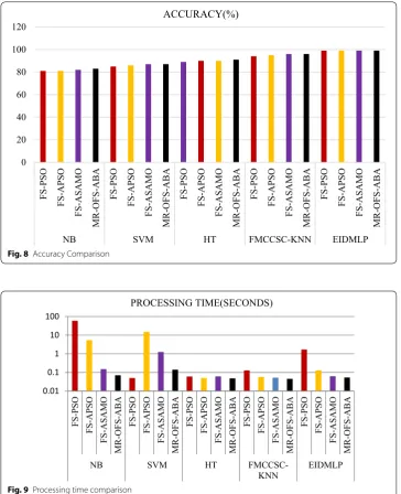
Figure 8 depicts the accuracy comparison of the MR-OFS-ABA with EIDMLP clas-sifier. The accuracy of arcene dataset to analyze the patient is affected with cancer or not is measured as 99%. The execution time is also shown in Fig. 9, as 0.053, 0.062, 0.13, and 1.68.
The performance metrics for the gisette dataset is shown in Table 3.
0 20 40 60 80 100 120
FS-PSO
FS-APSO
FS-ASAM
O
MR-OFS-ABA
FS-PSO
FS-APSO
FS-ASAM
O
MR-OFS-ABA
FS-PSO
FS-APSO
FS-ASAM
O
MR-OFS-ABA
FS-PSO
FS-APSO
FS-ASAM
O
MR-OFS-ABA
FS-PSO
FS-APSO
FS-ASAM
O
MR-OFS-ABA
NB SVM HT FMCCSC-KNN EIDMLP
ACCURACY(%)
Fig. 8 Accuracy Comparison
0.01 0.1 1 10 100
FS-PSO FS-APSO
FS-ASAM
O
MR-OFS-ABA
FS-PSO FS-APSO
FS-ASAM
O
MR-OFS-ABA
FS-PSO FS-APSO
FS-ASAM
O
MR-OFS-ABA
FS-PSO FS-APSO
FS-ASAM
O
MR-OFS-ABA
FS-PSO FS-APSO
FS-ASAM
O
MR-OFS-ABA
NB SVM HT
FMCCSC-KNN EIDMLP
PROCESSING TIME(SECONDS)
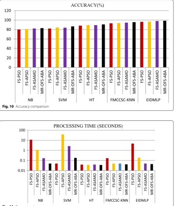
Figure 10 depicts the accuracy comparison of the MR-OFS-ABA with EIDMLP classifier. The accuracy of gisette to identify the digits 4 or 6 is measured as 98.6%, 98%, 96.7%, 96.3%. The execution time is also shown in presented in the Fig. 11, as 0.44, 0.05,0.19,4.72.
A receiver operating characteristic curve (ROC), is a graphical representation of classification model performance. The plot is drawn taking FPR, TPR along the axis x, y respectively. From the Fig. 12, the MROFS-ABA-EIDMLP curve is higher, thus proposed model performance is also higher.
0 20 40 60 80 100 120 FS-PSO FS-APS O FS-ASAMO MR-OFS-AB A FS-PSO FS-APS O FS-ASAMO MR-OFS-AB A FS-PSO FS-APS O FS-ASAMO MR-OFS-AB A FS-PSO FS-APS O FS-ASAMO MR-OFS-AB A FS-PSO FS-APS O FS-ASAMO MR-OFS-AB A
NB SVM HT FMCCSC-KNN EIDMLP
ACCURACY(%)
Fig. 10 Accuracy comparison
0.01 0.1 1 10 100 FS-PS O FS-APS O FS-ASAM O MR-OFS-AB A FS-PS O FS-APS O FS-ASAM O MR-OFS-AB A FS-PS O FS-APS O FS-ASAM O MR-OFS-AB A FS-PS O FS-APS O FS-ASAM O MR-OFS-AB A FS-PS O FS-APS O FS-ASAM O MR-OFS-AB A
NB SVM HT FMCCSC-KNN EIDMLP
PROCESSING TIME (SECONDS)
Conclusion
This paper focuses on innovative feature selection mechanism termed as OFS- Accel-erated Bat Algorithm (ABA) is proposed to choose the most important features from online streaming features. The proposed OFS-ABA algorithm employs MapReduce (MR) perception in a streaming method towards assessment of improving the run time among features. Lastly, Ensemble Incremental Deep Multiple Layer Percep-tron (EIDMLP) classifier is anticipated to classify dataset samples. The methodol-ogy is applied to three datasets and results were compared with four classifiers and three state-of-the-art feature selection algorithms. In this research work, MR-OFS-ABA method has shown improved performance than the existing feature selection methods namely PSO, APSO and ASAMO (Accelerated Simulated Annealing and Mutation Operator). The outcome of the EIDMLP classifier is compared with other prevailing classifiers such as Naïve Bayes (NB), Hoeffding tree (HT) and FMCCSC (Fuzzy Minimal Consistent Class Subset Coverage (FMCCSC)-KNN (K Nearest Neighbour). The upshot of this work has shown heightened performance in accuracy and less processing time. In big data analytics, it is really challenging to combat the all the characteristics of big data. Indeed, in the proposed model the Volume, Vari-ety, and Velocity is handled in a most proficient way. But, these characteristics may evolve into new dimensions in near future. The research challenge is to develop fea-ture selection model for upcoming challenges and complexities.
0 0.1 0.2 0.3 0.4 0.5 0.6 0.7 0.8 0.2
0.3 0.4 0.5 0.6 0.7 0.8 0.9 1
FPR
TP
R
EIDMLP FS-PSO EIDMLP FS-APSO EIDMLP FS-ASAMO EIDMLP MR-OFS-ABA
0 0.1 0.2 0.3 0.4 0.5 0.6 0.7 0.8 0.9 1 0.1
0.2 0.3 0.4 0.5 0.6 0.7 0.8 0.9 1
FPR
TP
R
EIDMLP FS-PSO EIDMLP FS-APSO EIDMLP FS-ASAMO EIDMLP MR-OFS-ABA
a
b
c
0 0.1 0.2 0.3 0.4 0.5 0.6 0.7 0.8 0.9 0.10.2 0.3 0.4 0.5 0.6 0.7 0.8 0.9 1
FPR
TP
R
EIDMLP FS-PSO EIDMLP FS-APSO EIDMLP FS-ASAMO EIDMLP MR-OFS-ABA
Abbreviations
OFS: Online Feature Selection; ABA: Accelerated Bat Algorithm; EIDMLP: Ensemble Incremental Deep Multiple layer Perceptron; MR: MapReduce; ML: machine learning; DL: deep learning; FS: feature selection; NLP: natural language pro-cessing; SVM: support vector machine; NB: Naïve Bayes; LR: logistic regression; PFBP: forward–backward with pruning; SIP: semi-infinite programming; MKL: multiple kernel learning; EC: evolutionary computation; SAOLA: Scalable and Precise Online Feature Selection; MOANOFS: Multi-Objective Automated Negotiation based Online Feature Selection; DMLP: Deep Multiple Layer Perceptron; HT: Hoeffding tree.
Acknowledgements Not applicable.
Authors’ contributions
Both authors read and approved the final manuscript.
Funding
No external funding.
Availability of data and materials
Datasets used in this work are available in UCI Machine Repository.
Competing interests
The authors declare that they have no competing interests.
Received: 12 August 2019 Accepted: 4 November 2019
References
1. AlNuaimi N, et al. Streaming feature selection algorithms for big data: a survey. Appl Comput Inform. 2019. https :// doi.org/10.1016/j.aci.2019.01.001.
2. Oussous Ahmed, et al. Big data technologies: a survey. J King Saud Univ Comput Inf Sci. 2018;30(4):431–48. 3. Dean J, Ghemawat S. MapReduce: simplified data processing on large clusters. Commun ACM. 2008;51(1):107–13. 4. Chu CT, Kim SK, Lin YA, Yu Y, Bradski G, Olukotun K, Ng AY. Map-reduce for machine learning on multicore. In:
Advances in neural information processing systems. p. 281–288; 2007.
5. Dean J, Ghemawat S. MapReduce: a flexible data processing tool. Commun ACM. 2010;53(1):72–7.
6. Athmaja S, Hanumanthappa M, Kavitha V. A survey of machine learning algorithms for big data analytics. In: Interna-tional conference on innovations in information, embedded and communication systems (ICIIECS). p 1–4; 2017. 7. Hinton GE, Osindero S, Teh Y-W. A fast learning algorithm for deep belief nets. Neural Comput. 2006;18(7):1527–54. 8. Bengio Y, Lamblin P, Popovici D, Larochelle H. Greedy layer-wise training of deep networks. In: Advances in neural
information processing systems. p. 153–160; 2007.
9. Dahl G, Ranzato M, Mohamed A-R, Hinton GE. Phone recognition with the mean-covariance restricted Boltzmann machine. In: Advances in neural information processing systems. Curran Associates, Inc; p. 469–77; 2010. 10. Krizhevsky A, Sutskever I, Hinton G. Imagenet classification with deep convolutional neural networks. In: Advances
in neural information processing systems, vol. 25. Curran Associates, Inc; p. 1106–1114; 2012.
11. Mikolov T, Deoras A, Kombrink S, Burget L, Cernock`y J (2011) Empirical evaluation and combination of advanced language modeling techniques. In: INTERSPEECH. ISCA. p. 605–608.
12. Saeys Y, Inza I, Larrañaga P. A review of feature selection techniques in bioinformatics. Bioinformatics. 2007;23(19):2507–17.
13. Liu H, Yu L. Toward integrating feature selection algorithms for classification and clustering. IEEE Trans Knowl Data Eng. 2005;17(4):491–502.
14. Hoi SC, Wang J, Zhao P, Jin R. Online feature selection for mining big data. In: Proceedings of the 1st international workshop on big data, streams and heterogeneous source mining: algorithms, systems, programming models and applications. p. 93–100; 2012.
15. Stefanowski J, Cuzzocrea A, Slezak D. Processing and mining complex data streams. Inf Sci. 2014;285:63–5. 16. Gill SS, Rajkumar B. Bio-inspired algorithms for big data analytics: a survey, taxonomy, and open challenges. In: Big
data analytics for intelligent healthcare management. Academic Press; p. 1–17; 2019.
17. Peralta D, del Río S, Ramírez-Gallego S, Triguero I, Benitez JM, Herrera F. Evolutionary feature selection for big data classification: a MapReduce approach. Math Prob Eng. 2015;2015:246139.
18. Tsamardinos I, Borboudakis G, Katsogridakis P, Pratikakis P, Christophides V. A greedy feature selection algorithm for Big Data of high dimensionality. Mach Learn. 2019;108(2):149–202.
19. Tan M, Tsang IW, Wang L. Towards ultrahigh dimensional feature selection for big data. J Mach Learn Res. 2014;15:1371–429.
20. de La Iglesia B. Evolutionary computation for feature selection in classification problems. Wiley Interdiscip Rev Data Min Knowl Discov. 2013;3:381–407.
21. Nazar NB, Senthilkumar R. An online approach for feature selection for classification in big data. Turk J Electr Eng Comput Sci. 2017;25(1):163–71.
22. Hu X, Zhou P, Li P, Wang J, Wu X. A survey on online feature selection with streaming features. Front Comput Sci. 2018;12(3):479–93.
24. Fong S, Wong R, Vasilakos A. Accelerated PSO swarm search feature selection for data stream mining big data. IEEE Trans Serv Comput. 2016;1:1–1.
25. Said FB, Alimi AM(2018) MOANOFS: Multi-objective automated negotiation based online feature selection system for big data classification. arXiv preprint arXiv :1810.04903 .
26. Lin KC, Zhang KY, Huang YH, Hung JC, Yen N. Feature selection based on an improved cat swarm optimization algorithm for big data classification. J Supercomput. 2016;72(8):3210–21.
27. Gu Shenkai, Cheng Ran, Jin Yaochu. Feature selection for high-dimensional classification using a competitive swarm optimizer. Soft Comput. 2018;22(3):811–22.
28. Manoj RJ, Praveena MA, Vijayakumar K. An ACO–ANN based feature selection algorithm for big data. Cluster Com-put. 2019;22:3953–60.
29. Devi SG, Sabrigiriraj M. A hybrid multi-objective firefly and simulated annealing based algorithm for big data clas-sification. Concurr Comput Pract Exp. 2019;31(14):e4985.
30. Wan S, Liang Y, Zhang Y, Guizani M. Deep multi-layer perceptron classifier for behavior analysis to estimate Parkin-son’s disease severity using smartphones. IEEE Access. 2018;6:36825–33.
31. Young S, Tamer A, Ayse B. Deep super learner: a deep ensemble for classification problems. In: Canadian conference on artificial intelligence. Springer, Cham; 2018.
32. Triguero I, Peralta D, Bacardit J, García S, Herrera F. MRPR: a MapReduce solution for prototype reduction in big data classification. Neurocomputing. 2015;150:331–45.
33. Chu CT, Kim SK, Lin YA et al. Map-reduce for machine learning on multicore. In: Advances in neural information processing systems. p. 281–288; 2007.
34. Yang XS. A new metaheuristic bat-inspired algorithm. In: Nature inspired cooperative strategies for optimization (NICSO 2010). Berlin: Springer; p. 65–74; 2010.
35. Yang XS, Hossein Gandomi A. Bat algorithm: a novel approach for global engineering optimization. Eng Comput. 2012;29(5):464–83.
36. Akhtar S, Ahmad AR, Abdel-Rahman EM. A metaheuristic bat-inspired algorithm for full body human pose estima-tion. In: Ninth conference on computer and robot vision. p. 369–75; 2012.
37. Renuka Devi D, Sasikala S. Accelerated simulated annealing and mutation operator feature selection method for big data. Int J Recent Technol Eng. 2019;8:910–6.
38. Fong S, Wong R, Vasilakos AV. Accelerated PSO swarm search feature selection for data stream mining big data. IEEE Trans Serv Comput. 2016;9(1):33–45.
39. Bouziane H, Messabih B, Chouarfia A. Profiles and majority voting-based ensemble method for protein secondary structure prediction. Evol Bioinform. 2011;7:EBO-S7931.
40. Sasikala S, Renuka Devi D. A review of traditional and swarm search based feature selection algorithms for handling data stream classification. In: Third international conference on sensing, signal processing and security (ICSSS), New York: IEEE; 2017.
Publisher’s Note