11
Technical sciences
The main output file when calculating the
displacement of the earth’s surface is differen-tial interferometer graph representing the result of
subtracting the synthesized phases of the topogra
-phy of integrated interferogram. Geocoding and
calibration are relative been obtained earlier
digi-tal elevation model of the city of Karaganda. The
calculations showed that in 2003 in the mine area Kostenko have started to form 2 of the mould of
subsidence. Up to 2010. mould concretion only in -crease. sedimentation are on average 2,5 cm during
the reporting period, i.e. approximately 30–50 days. On mine Kostenko currently conducted the work on formation K1 on the lava 45 K1-C capacity remov
-able reservoir made up 2,m/ Subsidence of a terres
-trial surface is calculated by the method of PSI, also showed subsidence in Kostenko mine area (fig. 1). Ac -cording to the schedule, sedimentation are active char-acter from 2003 to 2004-up to 80 mm 2005 to 2009 there is a small settlement in the region of 40 mm with
2009 is actively mining layer, which leads to an ac -tive process of displacement of the earth’s surface and subsidence of the mould displacement.
the interferogram of the Karaganda region shown
in fig. 3. (Processing of satellite images ENVISAT 2010/07/31 and 2010/10/09, subsidence of up to 5 cm).
Found subsidence on the undermined
territo-ries of the city of Karaganda indicate geodynamic processes, which may further lead to the destruction of asphalt pavement, paludification or flooding of land, and ultimately to failure. In this area it is nec
-essary to monitor the state of the earth’s surface to
predict the parameters of deformation and detection
References
1. Yavorskiy V.V., Moser D., Fofanov O. Space monitoring of man-made hazards in central Kazakhstan. // Mechanical En -gineering, Automation and Control Systems: Proceedings of In -ternational Conference, Tomsk, October 16–18, 2014. – Tomsk: TPU Publishing House, 2014 – Р. 1–5.
2. Arhipkin O.P., Spivak L.F., Sagatdinova G.N. Five years of experience in operational space monitoring of forest fires // modern problems of remote sensing earth from space. sat. sci-entific. articles. M: LLC “ABC-2000”, 2007.
3. Kudashev e.b., balashov A.D. integration of electronic libraries of satellite data into the international system of space data //Proceedings of the Fifth all-Russian scientific conference “digital libraries’03”. – S. Petersburg: Publishing house of St. PETERSBURG University, 2003.
4. Natural hazards in Russia. //Edited by Viekimova, Csa -gu. – M: Publishing house “KRUK”, 2001.
the work is submitted to the international
Scientific Conference “Prospects for the develop
-ment of university research”, Sochi, Russia, Oc
-tober 8–11, 2015, came to the editorial office оn 06.08.2015.
A new computAtionAl pAcKAge For using in cFD AnD other problems
mohammad reza Akhavan Khaleghi
The Office of Counseling and Research Fluid
Engineering and Aerodynamic, Mashhad, e-mail: [email protected]
First, i should mention that this is a basic pack-age and is not limited to cFD, it can also be used for other problems.
Finite element method (Fem) is a powerful
12
Technical sciences
for the solution of the existing problems in various scientific and engineering fields such as its applica
-tion in CFD. Many algorithms have been expressed
based on Fem, but none has been used in
popu-lar CFD software. In this section, full monopoly is
according to Finite volume method (Fvm) due to
better efficiency and adaptability with the physics
of problems in comparison with Fem. it doesn’t seem that Fem could compete with Fvm unless
it was fundamentally changed. In this paper, I am
going to show those changes and its result will be a powerful method which has much better perfor-mance in all subjects in comparison with Fvm and other computational method, i called it reduced Fi-nite element method (rFem).
the general form of a linear differential
equa-tion with boundary condiequa-tions can be shown as
follows [Zienkiewicz and morgan (1983);
Zienkie-wicz and Taylor (2001)]: RΩ =L φ+P
RΓ =M f+r (1)
the operators L and M in equations (1) can
be zero-order, odd-order, even-order or a combina-tion of two or all three
RW =Lf+ =P oddLf+evenLf+zeroLf+P
odd even zero
RΓ =M f+ =r Mf+Mf+Mf+r (2)
the weighted residual relationship for these
re-lationships on any element is
. .
eW R di Ω
Ω
Ω
∫
. .
eW R di Γ
Γ
Γ
∫
(3)And
. . . . 0
eW R di Ω eW R di Γ
Ω Γ
Ω + Γ =
∫
∫
(4)By inserting (2) in (3) we have
. .
e e e e
odd even zero
i i i i
W d W d W d W P d
Ω Ω Ω Ω
Ω + Ω + Ω + Ω
∫
∫
∫
∫
f f f
L L L
. . .
eWi d eW P di
Ω Ω
=
∫
L f Ω +∫
Ω (5). .
eWi d eWi d eWi d eW r di
Γ Γ Γ Γ
Γ + Γ + Γ + Γ
∫
odd∫
even∫
zero∫
f f f
M M M
. . . .
eWi d eW r di
Γ Γ
=
∫
M f Γ +∫
ΓThe approximate relation of the field also is equal to
. .0 M j j j N ∧ ∧ = ≈ =
∑
φ φ φ (6)
By inserting (6) in (5) we have
. .0 . .0 . .0
e e e
M M M
j j j
i j i j j
j j j
W N ∧d W N ∧ d W N ∧ d
Ω = Ω = Ω =
Ω + Ω + Ω
∑
∑
∑
∫
oddL φ∫
evenL φ∫
izeroL φ. . .
. . . .
e e e
M j j j
P d =
∑
N d P di i i
0
W W Ù W
W W W
W f W W
ò
ò
ò
=
+ L. + (7)
. . .
. .0 . .0 . .0
e e e
M M M
j j j
i j i j i j
j j j
W N ∧ d W N ∧ d W N ∧ d
Γ = Γ = Γ =
Γ + Γ + Γ
∑
∑
∑
∫
Modd φ∫
evenM φ∫
Mzero φ. . .0
. . . .
e e e
M j
i i j i
j
W r d W N ∧ d W r d
Γ Γ = Γ
+
∫
Γ =∫
M.∑
φ Γ +∫
ΓTogether all the elements a comprehensive system of equations is obtained which can be written quite generally as
..
13
Technical sciences
And
. .1 , . .1 .
e e
E E
ij ij i i
e e
K K f f
= =
=
∑
=∑
(9)Finally by using of equation (7) can write
e e
e
ij i j i j
K W N d W N d
Ω Γ =
∫
Ω +∫
Γ . . L M . . . . . e e ei i i
f W P d W r d
Ω Γ
= −
∫
Ω −∫
Γ
(10)
1 2 3
( , , ..., M)
∧ ∧ ∧ ∧
Τ ∧
=
φ φ φ φ φ
And this is the general form of approximation to a differential equation by the finite element method.
New Formulation for Finite
element method (nFFem)
Here I will introduce a new formulation for fi -nite element method which its performance is much
better than all conventional algorithms of finite ele -ment method in cFD. in nFFem relationship (9) is written as follows:
. .1 . ., . .1 .
e e
E E
ij ij i i
e e
K∗ K f∗ ∗ f∗
= =
=
∑
=∑
(11)And each of the matrix coefficients are
. . . .
e odd e even e zero e
ij ij ij ij
K∗= K ∗+ K ∗+ K ∗ (12)
where Kodd eij.
∗
become
( , , ) ( , , )
(1 ( ))
.
2 x y z x y z e
odd e odd
klm klm
ij i i i j
K ∗
b
W N dΩ
=
−
β−
β∫
Ω
L (13)
For even eKij.
∗
we have
( , , ) ( , , ) .
(1 ( ))
2
. x y z x y z e
even e even
klm klm
ij i i i j
K ∗
b
W L N dΩ
=
−
β−
β∫
Ω
(14)
For Kij.
∗ zero e
we have
( , , ) ( , , ) .
. (1 ( )) .
2 x y z x y z
e zero e
klm klm
ij i i i j
K ∗
b
W N dΩ
=
−
β−
β∫
Ω
(15)
And for fei∗. we have
( , , ) ( , , ) . .
(1 ( )
2
. x y z x y z)
e e
klm klm
i i i i
f∗
b
W P dΩ
=
−
β−
β∫
Ω (16)These relations are used for boundary integrals the same way, these are relations completely of NFFEM. In the equations (13) to (16), by choosing b = 1 full upwind difference scheme (FUDS) and by choos
-ing b = 0 central difference scheme (CDS) is obtained (Flux Vector Splitt-ing Methods (FVSM) can also use with NFFEM, in this form b = 1 is considered and equations are written separately for positive and
negative-terms after that the sum of the equations is done). these relationships are also valid for non-linear operators (
L
( )
φ
), which leads to Kije( )
∗
φ
. in the equations presented above, iklm( , , )x y z
β is given by
( ) ( ) ( ) ( ) ( ) ( ) ( , , )
( ) ( ) ( ) ( ) ( ) ( )
2( ) ( )
2( ) ( )
x y z x y z
x y z
x y z x y z
k l m k l m
klm
k l m k l m
i i i i i i
i
i i i i i i
+
+
−
+
+
=
+
+
−
+
+
β β β β β β ββ β β β β β (17)
For the central difference scheme the following equation can also be used instead of
( , , ) ( , , )
(1 ( ))
2 iklmx y z iklmx y z
b
−
β−
β in equations (13) to (16)( , , ) ( , , )
1
(1 ( ))
2 iklmx y z iklmx y z
−
β−
β (18)where iklm( , , )x y z
β is given by
( ) ( ) ( ) ( ) ( ) ( ) ( , , )
( ) ( ) ( ) ( ) ( ) ( )
( )
( )
x y z x y z
x y z
x y z x y z
k l m k l m
klm
k l m k l m
i i i i i i
i
i i i i i i
+
+
−
+
+
=
+
+
−
+
+
β β β β β β ββ β β β β β (19)
in this form, the number of participating elements in the equation of node i are limited to two elements
in 1D, 2D and 3D. the ik( )x
β , βil( )y and ( )z m
i
β are equal to
, ,
= = =
14
Technical sciences
where ( ) 0 0 , xk k k k
k
k k k k
i i L
i
i i L
x x x x
x x x x
− − = + − − β ( ) 0 0 y
l l l l
l
l l l l
i i L
i
i i L
y y y y
y y y y
− −
= +
− −
β (21)
( )
0
0
z
m m m m
m
m m m m
i i L
i
i i L
z z z z
z z z z
− −
= +
− −
β
And αi is the sign of the unknown variable or
derivations coefficients (any term that changes the sign of the matrix coefficients)
( )x x , x i A A = φ α φ ( ) , y y y i B B = φ α φ ( )z z
z i C C = φ α
φ (22)
Equation (17) can be written with βi and – βi
instead of the i
β that its result will be βiklm( , , )x y z , de-pending on the sign of βi that we have chosen, the
( , , )x y z klm
i
β gives the forward or backward
differenc-ing scheme.
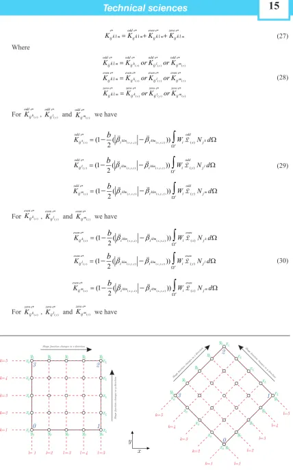
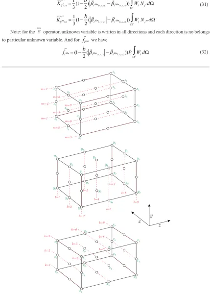
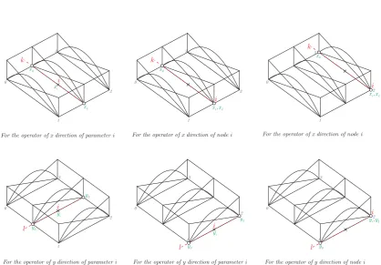
superscript k, l and m represent the terms are
located on lines k, l and m (the node i in three
di-mensions is located on three lines, line k at x
direc-tion, line l at y direction, and line m at z direction,
see figures (1) and (2)).
For hierarchical shape functions, the shape functions dependent to the sides and element as
shown in figures (3) and (4) attributable to the
points (these points as ξ η ζ0k, ,0l 0m, ξ η ζik, ,il im and , ,
k l m
L L L
ξ η ζ to calculate βi also to determine lines k, l and m are used).
when wind direction is constant before and
after discontinuity (shock), as an alternative (or as
another option for all position), βi′ can be used
in-stead of i
β , where βi′ is
( )x ( )x ( ),
k k x
i′ = i i′
β β α βi′l( )y =β αil( )y i′( )y, ( )z ( )z ( )
m m z
i′ = i i′
β β α . (23)
where
( )
2 0 2
. . . .
. . .
2 2
0 0
2 0 2
2 2
0 0 .
k k x k k e e L j j j j
j j L L
i e e
L
j j
j j
j j L L
N N x x N N x x + − + − ≥ ≤ ′ ≥ ≤ ∂ ∂ − ∂ ∂ = ∂ ∂ − ∂ ∂
∑
∑
∑
∑
φ φ α φ φ ( )2 0 2
. . . .
. . .
2 2
0 0
2 0 2
2 2
0 0 .
l l y l l e e L j j j j
j j L L
i e e
L
j j
j j
j j L L
N N y y N N y y + − + − ≥ ≤ ′ ≥ ≤ ∂ ∂ − ∂ ∂ = ∂ ∂ − ∂ ∂
∑
∑
∑
∑
φ φ α φ φ (24) ( )2 0 2
. . . .
. . .
2 2
0 0
2 0 2
2 2
0 0 .
m m z m m e e L j j j j
j j L L
i e e
L
j j
j j
j j L L
N N z z N N z z + − + − ≥ ≤ ′ ≥ ≤ ∂ ∂ − ∂ ∂ = ∂ ∂ − ∂ ∂
∑
∑
∑
∑
φ φ α φ φBecause βi is zero for internal nodes, there is no
need to calculate αi′, however it can be calculated
by the following equation
( ) 0 0 0 0 ,
k k k k
x
k k k k
i i i i i i i L L i i L L
x x x x
x x x x
′ − − − − − = − − − − − α
φ φ
φ φ
φ φ
φ φ
( ) 0 0 0 0l l l l
y
l l l l
i i i i i i i L L i i L L
y y y y
y y y y
′ − − − − − = − − − − − α
φ φ
φ φ
φ φ
φ φ
(25) ( ) 0 0 0 0m m m m
z
m m m m
i i i i i i i L L i i L L
z z z z
z z z z
′ − − − − − = − − − − − α
φ φ
φ φ
φ φ
φ φ
Note that NFFEM only for quadrilateral and hexahedron elements can be used. Solving the sys -tem of equations of the nFFem can be performed
simply by element by element solving method and line by line sweeping method.
reduced Finite element method (rFem)
A new method for the finite element formula -tion presented in the previous tion, in this sec-tion, i’m going to limit the participating nodes in equation for each node to the nodes that are located
on lines k, l and m the node. For this purpose, i
in-troduce reduced elements, characteristics of these elements is as follows:
1 – the different elements are used for different
directions of operator, see figures (5) and (6). 2 – For each direction of operator, element only
in the same direction has DoF (for one direction
of shape function is used p – degree function and
for other directions is used zero degree function, see
figures (5), (6), (7) and (8)).
3 – For equation of node i, element only on the
lines k, l and m the same node has the node, see
figures (7) and (8).
in rFem relationship (11) is written as follows:
.. ..
. .1
,
e k l m k l m
E
ij ij
e
K∗ K∗ =
=
∑
. .1
e klm klm
E
i i
e
f∗ f∗
=
=
∑
(26)
15
Technical sciences
..
e odd e even e zero e k l m k l m k l m k l m
ij ij ij ij
K∗ =K ∗ +K ∗+K ∗ (27) where ( ) ( ) ( ) ( ) ( ) ( ) ( )
x y z
x y z
x
odd e odd e odd e odd e
k l m k l m
even e even e even e even e
k l m k l m
zero e zero e k l m k
ij ij ij ij
ij ij ij ij
ij ij
K K or K or K
K K or K or K
K K o
∗ ∗ ∗ ∗ ∗ ∗ ∗ ∗ ∗ ∗ = = =
( )y ( )z zero e zero e
l m
ij ij
r K ∗ or K ∗
(28)
For ( )x
odd e k
ij
K ∗ , ( )y odd e
l
ij
K ∗ and ( )z odd e
m
ij
K ∗ we have
( ) ( , , ) ( , , ) ( )
.
(1 ( ))
2
k x x y z x y z
e
odd e odd
klm klm x k
ij i i i j
K ∗
b
W N dΩ =
−
β−
β∫
Ω L ( ) ( , , ) ( , , ) ( . )(1 ( ))
2
y x y z x y z
e
odd e odd
l klm klm y l
ij i i i j
K ∗
b
W N dΩ
=
−
β−
β∫
Ω
L (29)
( ) ( , , ) ( , , ) ()
.
(1 ( ))
2
z x y z x y z e
odd e odd
m klm klm z m
ij i i i j
K ∗
b
W N dΩ
=
−
β−
β∫
Ω
L
For ( )x
even e k
ij
K ∗ , ( )y even e
l
ij
K ∗ and ( )z even e
m
ij
K ∗ we have
( ) ( , , ) ( , , )
( ) .
(1 ( ))
2
x x y z x y z
e
even e even
k klm klm x k
ij i i i j
K ∗
b
W N dΩ =
−
β−
β∫
Ω L ( ) ( , , ) ( , , ) ( ) .(1 ( ))
2
y x y z x y z
e
even e even
l klm klm y l
ij i i i j
K ∗
b
W N dΩ
=
−
β−
β∫
Ω
L (30)
( ) ( , , ) ( , , )
( ) .
(1 ( ))
2
z x y z x y z
e
even e even
m klm klm z m
ij i i i j
K ∗
b
W N dΩ
=
−
β−
β∫
Ω
L
For ( )x
zero e k
ij
K ∗ , ( )y zero e
l
ij
K ∗ and ( )z zero e
m
ij
K ∗ we have
16
Technical sciences
Fig. 2. lines k, l and m on a quadratic element in three dimensions
( ) 1 (1 ( ( , , ) ( , , ))) . .
3 2
x x y z x y z
e zero e
k klm klm k
ij i i i j
K ∗
b
W N dΩ
=
−
β−
β∫
Ω
( ) 1 (1 ( ( , , ) ( , , ))) . .
3 2
y x y z x y z e
zero e
l klm klm l
ij i i i j
K ∗
b
W N dΩ
=
−
β−
β∫
Ω
(31)
( ) 1 (1 ( ( , , ) ( , , ))) .
3 2 .
z x y z x y z
e zero e
m klm klm m
ij i i i j
K ∗
b
W N dΩ
=
−
β−
β∫
Ω
note: for the zeroL operator, unknown variable is written in all directions and each direction is no belongs
to particular unknown variable. And for feiklm
∗
we have
( , , ) ( , , ) .
(1 ( ))
2 x y z x y z e
e
klm klm klm
i i i i i
f∗
b
P W dΩ
17
Technical sciences
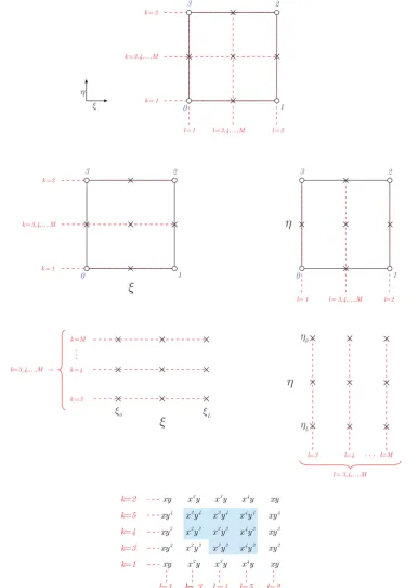
Fig. 3. Lines k and l also the places that β is calculated on for a hierarchical element in two dimensions
For approximating the mixed derivatives we will need to more DOF for example; if in three dimen
-sions, the mixed derivative be in two-direction, like following derivative
2 mix
xy x y x y
∂ = ∂ ∂ =
∂ ∂ ∂ ∂
φ φ
18
Technical sciences
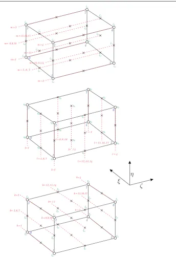
Fig. 4. Lines k, l and m also the places that β is calculated on for a fourth-degree hierarchical element in three
dimensions
we use the shape function with two DoF in x
and y directions, see figure (9). This elements are used only for mixed operator.
when we use the hierarchical shape functions,
for some equations have two unknown variable (ϕi
and ai, see figure (6)), the additional equation for
additional unknown can be written as follows: . .0 . .0 0
k k
L L
j i j j i j
j= N j= N a
+ + =
∑
φ∑
(34)19
Technical sciences
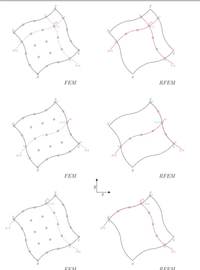
Fig. 5. A reduced standard quadratic element in two-dimensional, lines k and l also the participating nodes in the equation of node i for each of them
Fig. 6. A reduced hierarchical quadratic element in two-dimensional, lines k and l also the participating nodes in the
20
Technical sciences
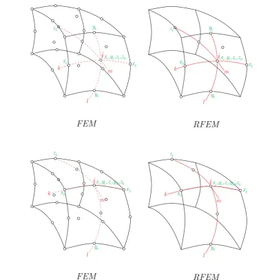
Fig. 7. nodes involved in the equation of node i for Fem and rFem on several fourth-degree elements in two dimensions
A new hybrid difference scheme (HDS) for liner shape functions
in this section, i will introduce a technique to eliminate oscillations for using the Fem and rFem
on liner shape functions, in this case b is written as
follows:
( , , )x y z
i
b=θ (35)
where θi( , , )x y z is “Upwind Parameter” and is
chosen in the range 0≤θi( , , )x y z ≤1. it is clear that there are many choices that can be used for. I used
21
Technical sciences
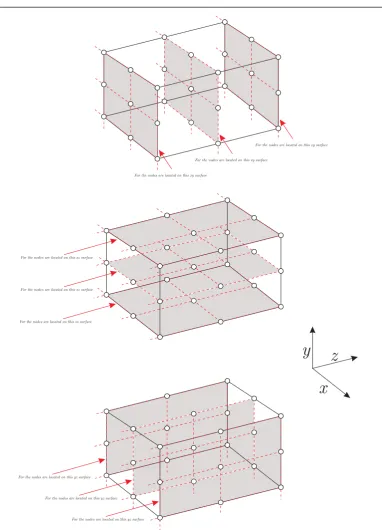
Fig. 8. nodes involved in the equation of node i for Fem and rFem on two quadratic elements in three dimensions
( , , ) ( , , )
7
(1
)
x y z iklmx y z
i
= −
rθ (36)
where
( , , )x y z min ( )x, ( )y, ( )z
klm k l m
i i i i
r = r r r (37)
And ( ) 1 1 1 1 1 1 1 1 min , max
,
,
xk k k k
k
k k k k
i i i i i i i i i i i i i i i i i
x x x x
r
x x x x
+ − + − + − + − − − − − = − − − −
φ
φ
φ φ
φ
φ
φ φ
( ) 1 1 1 1 1 1 1 1 min max,
,
yl l l l
l
l l l l
i i i i i i i i i i i i i i i
y y y y
r
y y y y
+ − + − + − + − − − − − = − − − −
φ
φ φ φ
φ
φ φ φ
(38)( ) 1 1 1 1 1 1 1 1 min max
,
,
zm lm m m m
m m m m
i i i i i i i i i i i i i i i i i
z z z z
r
z z z z
+ − + − + − + − − − − − = − − − −
φ
φ
φ φ
φ
φ
φ φ
the performance of this scheme is much better than other second-order schemes that in the Fem
are used for CFD, see figure (11).
A new shape functions for general problems
Equation (35) can be used only for the linear
shape functions, in this section another technique is provided for eliminating oscillations that can be
22
Technical sciences
, ( ) ( )
, ( ) ( )
, ( ) ( )
0 (1 ) 0 0
(1 )
(1 )
EDL FVL p ref
EDL FVL p ref
EDL FVL p ref
i i
i i
i i
j j j
L L L
N N N
N N N
N N N
= − +
= − +
= − +
δ δ
δ δ
δ δ
(39)
Where δi is element Degree limiter, Field
variable limiter (eDl, Fvl), and N(p) can be any
function of p ≥ 2 (for example, the functions of La
-grangian, Serendipity and Bezier for standard shape functions and the functions of Legendre, Cheby -shev, Fourier, etc. for hierarchical shape functions).
( )
0ref
N , (ref)
j
N and (ref)
L
N in equation (39) are
refer-ence functions, original function for them become
( ) (1)
0ref 0 ,
N =N (ref) 0,
j
N = (ref) (1)
L L
N =N (40)
where (1)
0
N and (1)
L
N are liner shape functions.
23
Technical sciences
The δi in equation (39) has two range:
1 – Using the δi as EDL by choosing it in the
range 0 EDL
i
<δ < ∞.
2 – Using the δi as FVL by choosing it in the
range FVL 0
i
− ∞ <δ < .
note: if the reference function is greater than the shape function the sign of eDl and Fvl will change.
The EDL can be used only in the directions
of the shape function (directions of operator) that
βi ≠ 0 is for, and the FVL is used only in the di
-rections of the shape function that βi = 0 is for or
inverse, or the Fvl and eDl can be added on all nodes with identical or non-identical values, and their relationship is written as follows:
(EDL FVL, )1 (1 ) (EDL FVL, )2
i = i i + − i i i
δ β δ β δ θ (41)
the value of the (EDL FVL, )1
i
δ and (EDL FVL, )2
i
δ
de-pending on the application is, see examples. Note that δi is applied to shape functions as
one-dimen-sional (separately for each direction of shape func -tions).
the following functions can also be used as
reference function on the Lagrangian, Serendipity
and bezier functions to make the shape functions of
non-oscillatory
( )
0ref L,
N =eN ( ) 0
0 ,
ref L
j j j L j
N =S N +S N +N
( )
0
ref
L
N =eN (42)
And for boundary elements become
( )
0ref 0 L,
N =N +eN (ref) L ,
j j L j
N =S N +N
(ref) 0
L
N = ( )
0ref 0,
N =
( ) 0
0 ,
ref
j j j
N =S N +N ( )
0
ref
L L
N =N +eN (43)
where e is a constant coefficient and N0, Nj and
NL can be the Lagrangian, Serendipity or Bezier
functions and degree them can be chosen 1 or p (for
1 – degree and p – degree the equations and results
are different). 0
j
S and L
j
S are a constant coefficients and are given by
. . 0 1 0 0 1 0 0 ,
(
)
(1 )
(
)
j j L j p j L S e = − − − = − − −∑
ω ωξ ξ
ξ ξ
ξ ξ
ξ ξ
. .1 0 1 0
(
)
(1 )
(
)
L L j j L j p j L L S e = − − − = − − −∑
ω ωξ ξ
ξ ξ
ξ ξ
ξ ξ
(44)Where ξj is the location of the nodes (control
points) and ω is the weight coefficient (optional).
For p ≥ 3 the hierarchical shape functions with
(ref) 0
j
N = can be used. e is chosen as, e = 1 – p for
ω = ∞, e = – 1 for ω = 0 and e = 1/1 – p for ω = – ∞.
Another reference function is
( )
0ref 1 (1 )(2 i 0 L)
N = +α N +eN
( ) 0
0
1 (1 ) (1 )
2
ref L
j i j L i j j
N = +α S N + −α S N +N
( )
0
1 (1 )( )
2
ref
i
L L
N = −α N +eN (45)
When αi = 1 equation (45) give backward dif
-ference approximation and when αi = – 1 give for
-ward difference approximation. A reference func -tion with high performance around discontinuities in derivative form is as follows:
. . ( ) ( ) ( ) ( ) 1 1 1 1 1 1 2 2 ref
k k k k
i i
i
i i i i
N ′ ′
− + + − ′ = − − − ξ ξ ξ α α
ξ ξ
ξ
ξ
. . ( ) ( ) 1( ) 1 1 1 2 ref k k i i i iN − ′
− + ′ = − − ξ ξ α
ξ ξ
. . ( ) ( ) 1( ) 1 1 1 2 ref k k i i i i N ′ + + − ′ = − ξ ξ αξ
ξ
. . ( )1 1( ) 0
ref
i i i
N′− > > + ξ =
. . ( ) ( ) ( ) ( ) 1 1 1 1 1 1 2 2 ref
l l l l
i i
i
i i i i
N ′ ′ − + + − ′ = − − − η η η α α
η η
η
η
. . ( ) ( ) 1( ) 1 1 1 2 ref l l i i i i N ′ − − + ′ = − − η η αη η
. . ( ) ( ) 1( ) 1 1 1 2 ref l l i i i i N ′ + + − ′ = − η η αη
η
. . ( )1 1( ) 0
ref
i i i
N′− > > + η = (46)
. . ( ) ( ) ( ) ( ) 1 1 1 1 1 1 2 2 ref
m m m m
i i
i
i i i i
N ′ ′
− + + − ′ = − − − ζ ζ ζ α α
ζ
ζ
ζ
ζ
. . ( ) ( ) 1( ) 1 1 1 2 ref m m i i i i N ′ − − + ′ = − − ζ ζ αζ
ζ
. . ( ) ( ) 1( ) 1 1 1 2 ref m m i i i i N ′ + + − ′ = − ζ ζ αζ
ζ
. . ( )1 1( ) 0
ref
i i i
N′− > > + ζ =
The difference between equation (46) and equa -tions (40), (42) and (45) on a fourth-degree element
24
Technical sciences
Fig. 10. The difference between equation (46) and equations (40), (42) and (45) on three fourth-degree elements around the discontinuity with FUDS
Fig. 11. liner functions for quadratic and cubic iGA functions
the r for higher-order shape functions is
writ-ten as re (the same for all nodes lines k, l and m)
( )x min 1( )x, 2 ( )x, 3( )x,..., 1( )x
k k k k k
e L
r = r r r r−
( )y min 1( )y, 2( )y, 3( )y,..., 1( )y
l l l l l
e L
r = r r r r− (47)
( )z min 1 ( )z , 2 ( )z ,3 ( )z,..., 1 ( )z
m m m m m
e L
r = r r r r−
where ri is given by equation (38).
New isogeometric analysis and new functions
In this section, I’m going by reference func -tions presented in the previous section, i introduce
a new isogeometric analysis. The isogeometric analysis [Hughes et al. (2005)] is done by the
B-spline and nurbs functions, although the refer-ence functions presented above are applicable with b-spline and nurbs functions, here i introduce a newIsogeometric Analysis Functions that are clos
-er to the standard finite element method and more
comfortable for the use in cFD and engineering, i made the following algorithm to make these func-tions on the bezier funcfunc-tions
( ) ( )
0IGA 12 0Bezier ,
N = N ( ) ( ) ( )
1IGA 12 0Bezier 1Bezier
N = N +N
. .
( ) ( )
2,3,4,...,IGA L 2 2,3,4,...,Bezier L 2
N − =N −
. .
( ) ( ) ( )
1 12 1 ,
IGA Bezier Bezier
L
L L
N − = N +N − NL(IGA) =12NL(Bezier) (48)
note that .
( )
2,3,4,...,IGA L 2
N − are local and can add as
hierarchical as well, for p = 2 these functions are
equivalent to the b-spline functions and for p = 3
are similar the pht-spline functions work of [Deng et al. (2008)] and for more than a third degree are
completely new. The equation (48) for first and last boundary elements become
( ) ( )
0IGA 0Bezier,
N =N ( ) ( )
1IGA 1Bezier
N =N
. .
( ) ( )
2,3,4,...,IGA L 2 2,3,4,...,Bezier L 2
N − =N −
. .
( ) ( ) ( )
1 12 1 ,
IGA Bezier Bezier
L
L L
N − = N +N − ( ) 1 ( )
2
IGA Bezier
L L
25
Technical sciences
( ) ( )
0IGA 12 0Bezier,
N = N ( ) ( ) ( )
1IGA 12 0Bezier 1Bezier
N = N +N ( ) . ( ) .
2,3,4,...,IGA L 2 2,3,4,...,Bezier L 2
N − =N −
. .
( ) ( )
1 1 ,
IGA Bezier
L L
N − =N − NL(IGA) =NL(Bezier) (50)
26
Technical sciences
Fig. 13. Euler equations 1D based on sod’s shock tube problem (t = 0.2)
For iGA functions, the liner functions to use
in equations (40), (42), (45) and (46) are a liner functions between two control points, see figure
(10), while the p-order functions for using in
27
Technical sciences
Fig. 14. Grid for flow around a cylinder
28
Technical sciences
Fig. 16. Mach contours for flow around a cylinder (steady-state Euler equations)
Solutions and Examples
In this section, some examples that have been solved by standard shape functions that
are including functions of the lagrangian and
bezier and hierarchical shape functions that are
including functions of the Legendre, Chebyshev (first and second kind) and Fourier Sine Se
29
Technical sciences
Fig. 17. Grid for flow over a NACA 0012 airfoil
Fig. 18. Surface skin friction coefficient distributions on NACA 0012 airfoil (steady-state Navier-Stokes equations) examples were solved to test RFEM is very high
and here are just a few of them select and
pre-sented. Examples include 1D advective equation,
1D and 2D euler equations, 2D navier – stokes equations and1D convection equation. here de-tails of the solution of these equations due to the
length of paper and be less important are not
pre-sented and only the results are shown. Note: All examples are RFEM (the results for the NFFEM is almost identical). I used the infinite elements for non-solid boundaries in all examples were
30
Technical sciences
31
Technical sciences
Fig. 20. Solution domain and lines grid for flat plate flow
32
Technical sciences
Fig. 22. 1D convection equation with source term, auх = сos(x) on [0, π] and a = 1
conclusions
the best criterion for evaluate a numerical meth-od is the results of the methmeth-od and as can be seen
in the examples were solved, the result of RFEM comparable to the best results were obtained by other methods is (for these examples, because of the small
size of the elements, the difference between the re-sults from different methods can not be seen) and
given that the system of equations resulting from this approach similar (in terms of density) Finite Differ
-ence Method (FDM) is its efficiency can be com
-pared with finite difference methods (although the use of the Legendre shape functions gives an effi
-ciency much higher than FDM) so do not think other
methods that are used in cFD be able to compete
with it. Also, due to the similarity of relations many
of the techniques used in the FDm can be used to rFem [hoffmann, and chiang (1998)].
References
1. Zienkiewicz o.c. and morgan K. Finite elements and Approximation, John Wiley & Sons, 1983.
2. Zienkiewicz O.C. and Taylor R.L. The Finite Element method: volume 1, the basis, butterworth-heinemann, 2001.
3. Laney C.B. Computational Gasdynamics. Publisher: Cambridge University Press. Pub. Date: June 28, 1998.
4. Hughes T.J.R, Cottrell J.A, Bazilevs Y. “Isogeometric analysis: CAD, finite elements, NURBS, exact geometry and mesh refinement”. Computer Methods in Applied Mechanics and Engineering, 194(39–41), Р. 4135–4195, 2005.
5. Hoffmann K.A. and Chiang, S.T. Computational Fluid Dynam -ics, Vol. I and II, 3rd edition, Engineering Education System (1998).
6. Deng J., Chen F., Li X., Hu C., Tong W., Yang Z. and Feng Y. Polynomial splines over hierarchical T-meshes. Graph. Models 70(4):76–86, 2008.
the work is submitted to the international
sci-entific Conference “Engineering science and mod
-ern manufacture”, France, October, 18–25, 2015, came to the editorial office оn 13.08.2015.
reseArch oF inFluence
OF MICRO-ARC OXIDATION MODES
on oxiDe coAting properties ramazanova Z.m., mustafa l.m. Joint-Stock Company “National Center of Space Research and Technology”, Almaty,
e-mail: [email protected]
Currently search for new efficient coatings with
high wear resistance, corrosion resistance, thermal resistance for spare parts of machines and mecha-nisms of different purpose is an ongoing process.
Due to the above a comparatively new method for treatment of valve metals surface – micro-arc oxi -dation method – is of interest. this method allows
obtaining fundamentally new coatings, which are characterized through different physical, chemical
and mechanical properties. pulse mode of
perform-ing micro-arc oxidation is of great interest. When forming oxide coating under the pulse mode by mi
-cro-arc oxidation method the value of current anode pulse duration has a significant impact on rough
-ness of the coating. The work studies influence of current anode pulse duration on properties of oxide coating obtained by micro-arc oxidation method.
Aluminum, titanium, zirconium alloys and other materials are widely used as structural materials in modern engineering and airspace industry. Search for new efficient coatings with high wear resistance,
corrosion resistance, thermal resistance for spare parts of machines and mechanisms of different pur-pose is an ongoing process. Due to this micro-arc
oxidation method (MAO) [1–3], which is compara
-tively new method for treatment of valve metals, is
of interest. the method allows obtaining brand new