Financial Time Series Forecasting Based on Characterized
Candlestick and the Support Vector Classification with
Cooperative Coevolution
Abstract:The fluctuations in prices in financial derivative market is an important indicator to a country or
region’s economic development, hence, predication of prices of financial derivatives is the research focus at present. However, the fluctuations in prices in financial market has high degree of nonlinearity, the traditional mathematical model has limitation to some extent, which influences the accuracy of prediction. This paper uses characterized Candlestick technique to implement noise removal processing on financial data and combines cooperative coevolution algorithms (CCEA) and support vector machine (SVM) to acquire the accuracy of classified prediction. After the noise removal processing made by characterized Candlestick technique, the core features of financial time series have been extracted, the randomness of financial data has been reduced, and the complexity of modeling has been simplified. The combination of CCEA and SVM has lifted the parameter optimization performance, acquired higher accuracy of classified prediction, and fit the solution of complex models. According to the computer simulation experiment, real stock data is used to verify the algorithm above, which has proved the high accuracy of prediction of this algorithm and the universality of this model.
Key words: Classified prediction, support vector machine, characterized candlestick, cooperative
coevolution algorithms.
1.
Introduction
The financial derivative market is influenced by politics, economy and participant's emotions. The system is highly nonlinear and has the characteristics of local randomness and global trend. Therefore, it is of great practical significance to track the trend of market movements and build the appropriate prediction model on this basis to effectively reduce the investment risk and raise the investment reward. With the continuous development of financial markets and improve, more and more high to the requirement of investors, early investors rely on their own subjective experience and judgment to make decisions to choose the speculation in the existing market conditions has been difficult to obtain a higher prediction accuracy. At the same time, with the rapid development of artificial intelligence technology represented by computer and machine learning, market prediction research based on financial data has become a hot spot in recent years.
SVM [1] is a classification technique proposed by Vapnik led by the experimental group based on
Jiang Zhipeng
1, Luo Chao
1,2,3*1School of Information Science and Engineering, Shandong Normal University, Jinan 250014, China.
2Shandong Provincial Key Laboratory for Novel Distributed Computer Software Technology, Jinan 250014,
China.
3Institute of Data Science and Technology, Shandong Normal University, Jinan 250014, China.
* Corresponding author. Email: [email protected]
statistical learning theory in 1995 [2]-[4], which is widely used in images [5], voice [6], natural language [7], [8] and other fields. Among them, SVM classification technology is also concerned in the field of financial
market forecasting. Kyong-jae et al. used SVM and reverse propagation neural network to predict financial
time series, which proved that SVM has the potential to deal with the prediction of financial time series [9].
Wang L et al. improved the performance of the prediction model by using SVM to predict the financial time
series by adding two-step kernel function [10]. He H and Starzyk J A combined SVM with self-organizing mapping to improve prediction classification accuracy [11]. Chi-jie Lu et al. used independent partial analysis method and SVM to predict financial time series, which improved the overall performance [12].
Candlestick graph [13] this chart source in Japan's tokugawa era, was Japanese rice market traders used to record the market price fluctuations and forecast, because of its good at capturing the time series model changes after core characteristics and was introduced into the stock market and futures market. At present, this kind of chart analysis is particularly popular in the asia-pacific region. The Candlestick is drawn at the opening, the highest, the lowest and the closing price of each analytical cycle. To draw the daily candlestick as an example, first determine the price of the opening and closing prices, and the parts between them are drawn as rectangular entities. If the closing price is higher than the opening price, the candlestick is called the positive line and is represented by a hollow entity. Instead, it is called a negative line with a black entity or a white entity. Characteristic Candlestick refers to the combination form of single root, two or multi-root Candlesticks with the same characteristics, and its occurrence tends to reflect a certain pattern of subsequent financial price movements. Financial derivatives market is affected by various factors, make the financial data, especially financial time series data of a large number of noise [14], cause the stability characteristics of time series, and greatly influenced on the analysis and processing. In view of the above situation, it is particularly important to work on the de-noising of financial time series. However, the financial time series itself has the characteristics of non-stationarity, non-linearity and high SNR, and the traditional de-noising method often has many defects. In this paper, the characteristic Candlestick based on financial time series data is used as the training data of classifier.
The traditional evolutionary algorithm has achieved good results in solving the problem of low dimension, and when the number of variables is small, the optimal solution can be found quickly. However, when the problem scale increases, the difficulty of solving the problem also increases dramatically, and many classical evolutionary algorithms lose their performance and performance in the low dimension. This is the so-called Curse of Dimensionality. Traditional classical algorithms have limitations in solving high-dimensional problems. Many optimization problems in practical engineering application are large scale, and there may be complex correlation between variables, so it is urgent to need effective and efficient large-scale optimization algorithm. Cooperative collaboration is one of the most effective strategies for improving the ability of evolution algorithm to solve high-dimensional problem [15]-[20].
Input multiple stock data, this article uses the trend s=0 or 1 of
the characteristic Candlestick
If s=1
Find out the 5 - day rising trading day
data
Find data on the 5 day falling trading
day
Yes No
Find out all specific form of transaction date data from the
data
The data of the characteristic Candlestick de-noising as the input
data of the SVM
Population P (P1, P2, P3,...Pn).The Pi is made up of three parts on the right.
SVM for the above n individual training prediction, get the prediction classification accuracy. Characteristic Candlestick denoising
Part 2: number of days window (5-30) Part 1: feature subset (random selection of feature subset from 21 features) part 3: optimization algorithm (1. Grid search 2.GA 3.PSO)
The individual with the highest accuracy was emperor, and the genetic algebra gen=0;gen=gen+1; set the maximum genetic algebra to
Gmax.
If gen>Gmax?
End, output emperor's classification accuracy. set the maximum genetic algebra to Gmax. Yes
The individual with the highest accuracy of prediction classification was emperor, and gen/3 took the remainder. No
In addition to emperor, the rest of the individual copies
the part 2 of emperor with the probability Pc, and the variation of part 2 is carried out with the probability Pm.
In addition to emperor, the rest of the individual copies
the part 3 of emperor with the probability Pc, and the variation of part 3 is carried out with the probability Pm. In addition to
emperor, the other individual copies the parts 1 of emperor with probability Pc, and the variation of part 1 is carried out with probability Pm.
If remainder =2
CC-SVM
If remainder =0 If remainder =1
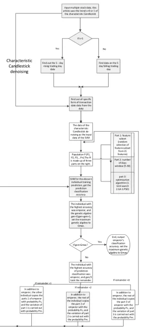
The main problem of this paper can be summarized as follows: on the basis of processing the characterized candlestick of financial data, and then combining the cooperative co-evolution algorithm with SVM, the prediction of financial time series is studied. Firstly, based on the candlestick of financial time series, the collection of characterized candlesticks with single root, double root and multiple roots is selected. Secondly, a financial time series prediction model is constructed based on the optimization framework constructed by cooperative collaborative evolution algorithm. The optimization framework mainly consists of three parts: feature subset, window length, optimization algorithm. Feature selection and Window length together determine the data set. The dataset has an impact on SVM optimization parameters c and g.It is simply not enough to optimize a single component individually without considering the interaction between them. However, all three problems are judged by the final classification accuracy as the only criterion. It is precisely because these three parts are closely related, this paper uses the cooperative coevolution method based on genetic algorithm (CCGA) to optimize the above three components. The validity of the proposed algorithm is verified by real stock data.
2.
Model
The model is shown in Fig. 1, which consists of two parts. The first part denotes the characterized candlestick, and the second part is CC-SVM.
2.1.
Methods of De-noising
Traditional methods of de-noising financial time series are mainly moving average method [31], traditional filtering method [32], Kalman filtering method [33] and wiener filtering method [34]. As a kind of simple moving average method of data smoothing techniques, this method is very rough, while de-noising, a lot of useful information was also removed, so it is only for simple analysis of the data, not suitable for the deep analysis of the data. Traditional filtering requires that the spectrum of useful signals and noise be separated from each other. But for financial time series, such as stock price time series and its volatility yield sequence are bigger, the spectrum is wide, and the useful signal and noise spectrum overlap is serious, the traditional method is difficult to achieve effective separation of signal-to-noise. Kalman filter needs to know the motion of the system to establish an accurate equation of state. But the financial time series is a non-stationary and nonlinear time series, it is difficult to use a certain equation to describe the state and behavior, therefore this method is used to de-noising of financial time series is the inherent difficulty. Wiener filter requires prior knowledge of noise and useful signals such as their autocorrelation function and power spectral density. Because these prior knowledge is difficult to be obtained or oversimplified in practice, the optimal wiener filter is often not required. The complexity, variability and non-linearity of financial time series increase the difficulty of forecasting. The particularity of time series prediction has the limitation of traditional de-noising method.
Technical analysis refers to financial derivatives prices rise and fall of intuitive behavior as the main research object, to predict price movements form and trend for the main purpose, from the candlestick chart and technical indexes of stock price changes, analyze the law of stock market volatility method combined. Technical analysis to predict financial time series, often appears in a certain feature of candlestick as the basis of market trends, such as in the downward trend of Inverted hammer, the herald the end of the downward trend. The appearance of Hanging man in the rising trend indicates the end of the upward trend. Therefore, as shown in Fig. 1, the characterized candlestick de-noising part, taking out the same characterized candlestick in the same trend as the training data of classifier, is also the de-noising method of this paper. This characterized candlestick de-noising method originates from the traditional technical index analysis.
occurrence of singular value is usually caused by sudden events, which usually indicates the end of trend or the enhancement of trend. Therefore, the singular value is not noise, but is research focus. The characterized candlestick fully embodies the value of the singular value. Due to the particularity of financial time series prediction, traditional de-noising method does not apply. Compared with traditional de-noising methods, the characteristics of candlestick de-noising method not only reduces the amount of data, reduce the complexity of the classified prediction, and improve the classification accuracy to a great extent, it will be in the back of the validating experiment part.
2.2.
The Use of Cooperative Coevolution Algorithm in SVM (CC-SVM)
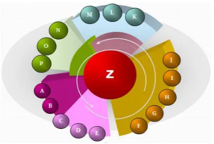
The idea of collaborative evolution using biological coevolution. By constructing multiple species and establishing the relationship between them, multiple species can improve their performance to achieve the goal of population optimization. The individuals of A-P in Fig. 2 are both useful to the final result, Z, and interact with each other. In this case, it's just A-P looking for their optimal solution, and obviously you can't get the optimal solution for Z. Accordingly, it presents the method of cooperative coevolution, cooperative coevolution is defined like this: by constructing multiple populations and to establish the relationship between them, multiple population to improve their performance by interaction, to adapt to the dynamic evolution of complex system environment, to achieve the goal of population optimization. The relationship between all individuals of A-P is established to adapt to the complex dynamic evolution environment and obtain a better solution of Z.
Fig. 2. Example diagram of cooperative collaborative evolution algorithm.
As shown in Fig. 1, the cooperative coevolution and support vector machine section contains feature subset, window length, optimization algorithm. Feature subset selection, from the following characteristics of DIF, DEA, MACD, DMA, AMA, PSY, CLOSE, D, RSI, OPEN, HIGH, MA5, MA10, VOLUME, K, LOW, UPPERLINE, MIDDLELINE, LOWLINE, CCI, j feature subset is selected. window length, randomly select between 5 days and 30 days. Optimization algorithm, random selection of values between 1 and 3, 1 represents grid search, 2 represents GA algorithm, and 3 represents particle swarm algorithm. In this paper, the cooperative collaborative evolutionary algorithm (CCGA) based on genetic algorithm is used to optimize these three problems. Here's how:
50 individuals get their respective SVM classification accuracy, choose the highest classification accuracy of the individual as emperor, gen = gen+1, if gen/3 of the remainder is 1, Other individuals copy the emperor's first component with probability Pc, self mutation with probability Pm. 50 individuals get their respective SVM classification accuracy, choose the highest classification accuracy of the individual as emperor, gen = gen+1, if gen/3 of the remainder is 2, other individuals copy the emperor's second component with probability Pc, Self mutation with probability Pm. 50 individuals get their respective SVM classification accuracy, choose the highest classification accuracy of the individual as emperor, gen = gen + 1, if gen/3 of the remainder is 0, other individuals copy the emperor's third component with probability Pc, Self mutation with probability Pm.until the number of cycles is reached. Record feature subset, window length and optimization algorithm of emperor. The classification prediction accuracy of emperor is the correct classification prediction accuracy.
Cooperative coevolution algorithm and the code used by SVM:
gen = 0
for each species s do begin
Pops (gen) = randomly initialized each species’ three subcomponents
end
while gen < maximum number of generations do begin
gen = gen+1
calculate accuracy of each species by CC-SVM in Pops (gen)
emperor = the species with maximum accuracy for each species s do begin
remainder = s%3
the remainder ‘s subcomponent of each species in a Pc probability= the remainder ‘s subcomponent of emperor
self variation of the remainder ‘s subcomponent of each species in a Pm probability
end end
3.
Experiments
3.1.
Experimental Design
Feature candlestick de-noising: in order to better verify our proposed method in financial market, extract data from 3612 different stock data. These financial data are taken from Wind and other public channels. In order to establish our trading model, the obtained financial data needs to be de-noised. We use the method of selecting characterized candlesticks from the data to process the financial time series. Take the candlesticks of all the same forms in the time series and their associated data. For example, select all the Inverted hammer in the downward trend. n days data as dataset. Select m from the following indicators: DIF DEA MACD DMA AMA PSY CLOSE D RSI HIGH OPEN MA5 MA10 VOLUME LOW K UPPERLINE MIDDLELINE LOWLINE CCI J. Both m and n need to be selected in the process of SVM training test. Compared with the data that is not de-noised, the data volume with the characterized candlestick de-noising is smaller, and the classification accuracy is higher. When comparing the experiment, the data of the same size as the above experiment was selected randomly.
The dataset will be divided into two parts, the training set and the test set. The first 200 sets of data sets are used as training sets and the latter 1000 sets as test sets. The superiority of the characterized candlestick de-noising is verified by experiment.
algorithm. The usual approach is to look for the best parts one by one. This approach does not take into account the relationship between components, and the best of each component is not globally optimal. The cooperative coevolution algorithm will optimize the above three parts. The experimental results show that the cooperative coevolution is applied to SVM, and the classification accuracy is higher. Let's say that the number of cycles is C, N individuals constitute a population, feature subset, window length, optimization algorithm to be determined, day is the number of days, fea represents a subset of features, and opt represents the choice of optimization algorithm. Initialize the first k individuals, the extraction of day is a random value between 5-30, fea is randomly take out the characteristics of 21 feature subset, which is take out the several characteristics and here several characteristics are random. Opt is a random number between 1-3, representing grid algorithm, genetic algorithm, particle swarm algorithm. Based on the three components of each individual in the population, the SVM based on the candle chart combines the characterized candlestick to noise, and CCEA and SVM can work together to get the accuracy.
Three components and accuracy are obtained as follows:
1, 2, 3...
.
(5 30)
.
.
(1 3)
.
(
)
k
k day
k fea
k opt
k acc k
P k
N
P
rand
P
a random subset of feature set
P
rand
P
CCEA SVM P
After the initialization is completed, each individual's feature subset, window length, optimization algorithm and accuracy will be obtained. The first three components of the cooperative coevolution algorithm are part 1, part 2, and part 3. Accuracy as fitness. N individuals make up a population. Remove the highest accuracy of individuals for the emperor. If the current number of cycles C/3 remainder is 1, except emperor, component 1 of the rest of the individual will be copied into component 1 of emperor according to the crossover rate Pc, and then the variation of component 1 will be carried out according to the mutation rate Pm. Then calculate the accuracy of each individual, take out the highest accuracy of the individual is emperor, if the current number of cycles C/3 remainder is 2, except emperor, the rest of the individual parts 2 will be copied according to the crossover rate of Pc into emperor parts 2, after the completion of the copy, then according to the variation rate of Pm for their own variation. Then calculate the accuracy of each individual, the highest accuracy of the individual is emperor, if the current number of cycles C/3 remainder is 0, then the other individual parts 3 will be copied into emperor parts 3 according to the crossover rate Pc, and then according to the mutation rate Pm to make their own variation. Reaching the maximum number of cycles, the last emperor is the individual we want.
3.2.
Experimental Results
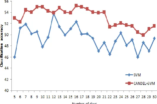
1) Comparison test between SVM and CANDEL+SVM to obtain the highest classification prediction accuracy step by step.
In the way of CANDEL+SVM, the first 200 sets of data are used as training sets, and the latter 1000 sets of data are used as test sets. The way of SVM is to randomly select the amount of data roughly equivalent to CANDEL+SVM from stock data.
first 14 feature sets of feature subset, obtained the highest classification accuracy of 52. 5090%. The de-noising of feature candlestick is helpful for obtaining higher classification accuracy. The feature set includes the DIF DEA MACD DMA AMA CLOSE D RSI HIGH OPEN MA5 MA10 VOLUME K LOW UPPERLINE MIDDLELINE LOWLINE CCI J, in order to rank the above features 1-21. If DIF DEA MACD DMA is taken out, it is expressed as 1. 2. 3. 4 in the table. The feature subset of the two methods is shown in Table 1. At this point, the number of days window is 1, and the optimization algorithm selects the grid search algorithm in LIBSVM.
Fig. 3. Variation of classification accuracy with subsets.
Table 1. The Corresponding Feature Subset of the Optimal Classification Accuracy
feature subset Accuracy%
SVM 12. 3. 4. 5. 6. 7. 8. 9. 10. 11. 12. 13. 14 52. 5090
SVM+CANDEL 1. 2. 3. 4. 5. 6. 7 53. 8740
Number of days window setting: As shown in Fig. 4, SVM+CANDEL obtained the maximum classification accuracy of 55. 1537% at n=16. SVM, the maximum classification accuracy at n=12 was 53. 7634%. At this time, the feature subset is in Table 1, and the optimization algorithm is the grid search by LIBSVM.
Fig. 4. Variation of the classification prediction accuracy with the number of days.
accuracy =53. 7634% when n=1 and select grid search. At this time, the feature subset is in Table 1, the number of days window of SVM is taken from the 12 obtained from 2. 2, and the window size of SVM+CANDEL is taken from the 16 obtained from 2. 2.
Fig. 5. The influence of three optimization algorithms on accuracy.
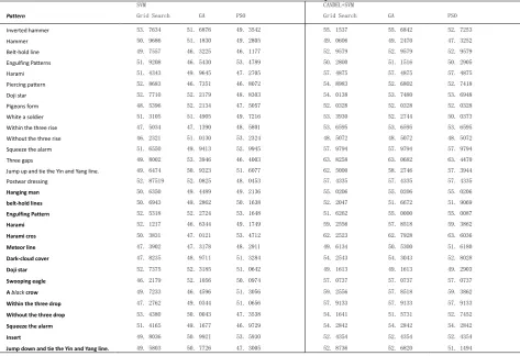
Table 2. SVM and CANDEL+SVM in 30 Different Feature Candlesticks, Three Optimization Algorithms Predict Classification Accuracy
SVM CANDEL+SVM
Pattern Grid Search GA PSO Grid Search GA PSO
Inverted hammer 53. 7634 51. 6876 49. 3542 55. 1537 55. 6842 52. 7253
Hammer 50. 9686 51. 1830 49. 2805 49. 0606 49. 2470 47. 3252
Belt-hold line 49. 7557 46. 3225 46. 1177 52. 9579 52. 9579 52. 9579
Engulfing Patterns 51. 9208 46. 5430 53. 4789 50. 2800 51. 1516 50. 2905
Harami 51. 4343 49. 9645 47. 2705 57. 4875 57. 4875 57. 4875
Piercing pattern 52. 8683 46. 7351 46. 8072 54. 8983 52. 6802 52. 7418
Doji star 52. 7710 52. 2179 48. 8303 54. 0138 53. 7480 53. 6948
Pigeons form 48. 5396 52. 2134 47. 5057 52. 0328 52. 0328 52. 0328
White a soldier 51. 3105 51. 4905 49. 7216 53. 3930 52. 2744 50. 0373
Within the three rise 47. 5034 47. 1390 48. 5801 53. 6595 53. 6595 53. 6595
Without the three rise 46. 2321 51. 0130 53. 2324 48. 5072 48. 5072 48. 5072
Squeeze the alarm 51. 6550 49. 9413 52. 9945 57. 9794 57. 9794 57. 9794
Three gaps 49. 8002 53. 3946 46. 4003 63. 8258 63. 0682 63. 4470
Jump up and tie the Yin and Yang line. 49. 6474 50. 9323 51. 6077 62. 5000 58. 2746 57. 3944
Postwar dressing 52. 87519 52. 0825 48. 0453 57. 4335 57. 4335 57. 4335
Hanging man 50. 6350 49. 4489 49. 2136 55. 0206 55. 0206 55. 0206
belt-hold lines 50. 6943 49. 2862 50. 1638 52. 2047 51. 6672 51. 9069
Engulfing Pattern 52. 5318 52. 2724 53. 1648 51. 6262 55. 0000 55. 0087
Harami 52. 1217 46. 6344 49. 1749 59. 2556 57. 8518 59. 3862
Harami cros 50. 3831 47. 0121 53. 4712 62. 2523 62. 7928 63. 6036
Meteor line 47. 3902 47. 3178 48. 2911 49. 6134 50. 5300 51. 6180
Dark-cloud cover 47. 8235 48. 9711 51. 3284 54. 2543 54. 3043 52. 8028
Doji star 52. 7375 52. 3185 51. 0642 49. 1613 49. 1613 49. 2903
Swooping eagle 46. 2179 52. 1056 50. 0974 57. 0737 57. 0737 57. 0737
A black crow 49. 7233 46. 4596 51. 3056 59. 2556 57. 8518 59. 3862
Within the three drop 47. 2762 49. 0344 51. 0656 57. 9133 57. 9133 57. 9133
Without the three drop 53. 4380 50. 0043 47. 3538 54. 1641 51. 5731 52. 7452
Squeeze the alarm 51. 4165 49. 1677 46. 9729 54. 2842 54. 2842 54. 2842
Insert 49. 8036 50. 9921 53. 5930 52. 4354 52. 4354 52. 4354
Jump down and tie the Yin and Yang line. 49. 5803 50. 7726 47. 3005 52. 8736 52. 6820 51. 1494
and the latter 15 are bearish patterns in the rising trend (bold, diagonal).
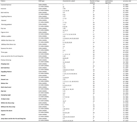
The following Table 3 is the selected feature subset, number of days window and optimization algorithm in the prediction of 30 characterized candlesticks. The first 15 are bullish in the downward trend, and the latter 15 are bearish patterns in the rising trend (bold, diagonal). The feature set includes the DIF DEA MACD DMA AMA CLOSE D RSI HIGH OPEN MA5 MA10 VOLUME K LOW UPPERLINE MIDDLELINE LOWLINE CCI J, in order to rank the above features 1-21. If DIF DEA MACD DMA is taken out, it is expressed as 1. 2. 3. 4 or 1-4 in the table.
Table 3. 30 Different Morphologies, Respectively in SVM+CANDEL and CC-SVM +CANDEL, Finally Acquired the Feature Subset, Number of Days Window, Optimization Algorithm and Accuracy
Pattern SVM type characteristic subset Number of days
window
optimization algorithm
accuracy rate
Inverted hammer SVM+CANDEL 1 18 1 55. 6842
CC-SVM+CANDEL 16 28 2 55. 9364
Hammer SVM+CANDEL 1-20 28 2 49. 2470
CC-SVM+CANDEL 1 11 15 19 28 1 55. 7000
Belt-hold line SVM+CANDEL 1-6 2 1 52. 9579
CC-SVM+CANDEL 4 16 30 2 53. 0909
Engulfing Patterns SVM+CANDEL 1-17 25 2 51. 1516
CC-SVM+CANDEL 1 7 15 29 2 57. 2222
Harami SVM+CANDEL 1 1 1 57. 4875
CC-SVM+CANDEL 1 7 15 26 1 56. 6250
Piercing pattern SVM+CANDEL 1-13 29 1 54. 8983
CC-SVM+CANDEL 6 10 20 29 1 56. 8000
Doji star SVM+CANDEL 1-20 19 1 54. 0138
CC-SVM+CANDEL 13 15 17 26 1 56. 7000
Pigeons form SVM+CANDEL 1-7 1 1 52. 0328
CC-SVM+CANDEL 1 2 3 7 11 12 14 15 20 27 2 58. 4000
White a soldier SVM+CANDEL 1-21 16 1 53. 3930
CC-SVM+CANDEL 1,7,8,10,11,14,15,18,19,20 27 2 58. 3000
Within the three rise SVM+CANDEL 1-7 1 1 53. 6595
CC-SVM+CANDEL 5,7,16,18,19,20 29 1 57. 3000
Without the three rise SVM+CANDEL 1-5 1 1 48. 5072
CC-SVM+CANDEL 1,4 26 1 54. 7000
Squeeze the alarm SVM+CANDEL 1 1 1 57. 9794
CC-SVM+CANDEL 2,11 30 2 58. 7273
Three gaps SVM+CANDEL 1 22 1 63. 8258
CC-SVM+CANDEL 1 – 9, 11- 21 26 3 64. 6250
Jump up and tie the Yin and Yang line. SVM+CANDEL 1-10 23 1 62. 5000
CC-SVM+CANDEL 4,8,16,20 26 1 66. 1250
Postwar dressing SVM+CANDEL 1-6 1 1 57. 4335
CC-SVM+CANDEL 11,13,14,20 29 3 58. 7000
Hanging man SVM+CANDEL 1-9 1 1 55. 0206
CC-SVM+CANDEL 5,15 26 1 57. 7000
belt-hold lines SVM+CANDEL 1-19 4 1 52. 2047
CC-SVM+CANDEL 1,4,6,8,15,17,18,21 28 1 53. 8000
Engulfing Pattern SVM+CANDEL 1 2 3 17 3 55. 0087
CC-SVM+CANDEL 1 -10 ,12 13 14 16 20 21 30 1 57. 5000
Harami SVM+CANDEL 1-7 30 3 59. 3862
CC-SVM+CANDEL 1,2,4,6,14 30 2 55. 5000
Harami cros SVM+CANDEL 1-21 29 3 63. 6036
CC-SVM+CANDEL 1 -5, 8, 11 -15, 18 19 20 21 26 1 63. 3000
Meteor line SVM+CANDEL 1-6 29 3 51. 6180
CC-SVM+CANDEL 5,7,9,11,12,13 28 1 56. 2000
Dark-cloud cover SVM+CANDEL 1-21 19 2 54. 3043
CC-SVM+CANDEL 2-8 ,10, 11 -18, 20 26 1 54. 5000
Doji star SVM+CANDEL 1-21 26 3 49. 2903
CC-SVM+CANDEL 1,11 30 2 56. 2000
Swooping eagle SVM+CANDEL 1-5 1 1 57. 0737
CC-SVM+CANDEL 3 7 9 15 16 30 1 58. 3886
A black crow SVM+CANDEL 1- 7 30 3 59. 3862
CC-SVM+CANDEL 13,17 29 1 61. 8000
Within the three drop SVM+CANDEL 1-9 1 1 57. 9133
CC-SVM+CANDEL 3 26 1 60. 6000
Without the three drop SVM+CANDEL 1-7 19 1 54. 1641
CC-SVM+CANDEL 1-18 ,20 21 30 2 59. 4000
Squeeze the alarm SVM+CANDEL 1-7 1 1 54. 2842
CC-SVM+CANDEL 3,5,9,11,20 28 1 55. 0000
Insert SVM+CANDEL 1-6 1 1 52. 4354
CC-SVM+CANDEL 5,10,12,14,15,18,19 26 1 59. 3000
Jump down and tie the Yin and Yang line. SVM+CANDEL 1-5 3 1 52. 8736
CC-SVM+CANDEL 2,5,6,11,13,14,15 29 2 57. 2222
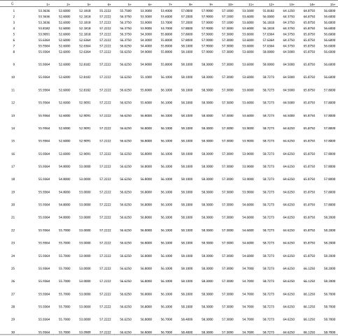
In CANDEL+ CC-SVM, with the increase of genetic algebra, the prediction accuracy rate of the 30 characterized candlesticks was changed as follows. Bullish in the downward trend lines to Inverted hammer, Hammer, Belt-hold line, Engulfing Patterns, Harami, Piercing pattern, Doji star, Pigeons form, White a soldier, Within the three rise, Without the three rise, Squeeze the alarm, Three gaps, Jump up and tie the Yin and Yang line, Postwar dressing, respectively, with 1 + 2 +, 3 +. . . 15 + said. With the increase of the cyclic algebra G, the change of accuracy is shown in Table 4. Bearish in the rising trend of Hanging man, Belt-hold
lines, Engulfing Pattern, Harami, Harami cros, Meteor line, Dark-cloud cover, Doji star, Swooping eagle, A black crow, Within the three drop, Without the three drop, Squeeze the alarm, Insert, Jump down and tie the Yin and Yang line, respectively, with 1 -, 2 -, 3 -. . . 15 - said. With the increase of the cyclic algebra G, the change of accuracy is shown in Table 5.
Table 4. Shows the 15 Characterized Candlesticks of the Rising Trend, and the Accuracy Changes with the Increase of Iteration Number G
G 1+ 2+ 3+ 4+ 5+ 6+ 7+ 8+ 9+ 10+ 11+ 12+ 13+ 14+ 15+ 1 53.3636 52.6000 52.1818 55.2222 55.7500 53.3000 53.4000 57.0000 57.9000 57.1000 53.5000 55.8182 64.1250 64.8750 56.6000 2 53.3636 52.6000 52.1818 57.2222 56.3750 53.3000 53.6000 57.2000 57.9000 57.1000 53.6000 56.0000 64.3750 64.8750 56.6000 3 53.3636 52.6000 52.1818 57.2222 56.3750 53.9000 53.7000 57.2000 57.9000 57.1000 53.6000 56.1818 64.3750 65.8750 56.6000 4 53.8182 52.6000 52.1818 57.2222 56.3750 53.9000 53.7000 57.8000 57.9000 57.3000 53.6000 56.1818 64.3750 65.8750 56.6000 5 53.9091 52.6000 52.1818 57.2222 56.3750 54.3000 55.8000 57.8000 57.9000 57.3000 53.6000 57.6364 64.3750 65.8750 56.6000 6 55.6364 52.6000 52.6364 57.2222 56.3750 54.3000 55.8000 57.8000 57.9000 57.3000 53.6000 57.6364 64.3750 65.8750 56.6000 7 55.9364 52.6000 52.6364 57.2222 56.6250 54.4000 55.8000 58.1000 57.9000 57.3000 53.6000 57.6364 64.3750 65.8750 56.6000 8 55.9364 52.6000 52.6364 57.2222 56.6250 54.9000 55.8000 58.1000 57.9000 57.3000 53.6000 58.0000 64.5000 65.8750 56.6000
9 55.9364 52.6000 52.8182 57.2222 56.6250 54.9000 55.8000 58.1000 58.3000 57.3000 53.6000 58.0000 64.5000 65.8750 56.6000
10 55.9364 52.6000 52.8182 57.2222 56.6250 55.1000 56.1000 58.1000 58.3000 57.3000 53.6000 58.7273 64.5000 65.8750 56.6000
11 55.9364 52.6000 52.8182 57.2222 56.6250 55.6000 56.1000 58.1000 58.3000 57.3000 53.6000 58.7273 64.5000 65.8750 57.8000
12 55.9364 52.6000 52.9091 57.2222 56.6250 55.6000 56.1000 58.1000 58.3000 57.3000 53.6000 58.7273 64.5000 65.8750 57.8000
13 55.9364 52.6000 52.9091 57.2222 56.6250 56.8000 56.1000 58.1000 58.3000 57.3000 53.6000 58.7273 64.5000 65.8750 57.8000
14 55.9364 52.6000 52.9091 57.2222 56.6250 56.8000 56.1000 58.1000 58.3000 57.3000 53.9000 58.7273 64.6250 65.8750 57.8000
15 55.9364 52.6000 52.9091 57.2222 56.6250 56.8000 56.1000 58.1000 58.3000 57.3000 53.9000 58.7273 64.6250 65.8750 57.8000
16 55.9364 52.6000 52.9091 57.2222 56.6250 56.8000 56.1000 58.1000 58.3000 57.3000 53.9000 58.7273 64.6250 65.8750 57.8000
17 55.9364 54.8000 53.0000 57.2222 56.6250 56.8000 56.1000 58.1000 58.3000 57.3000 53.9000 58.7273 64.6250 65.8750 57.8000
18 55.9364 54.8000 53.0000 57.2222 56.6250 56.8000 56.1000 58.1000 58.3000 57.3000 53.9000 58.7273 64.6250 65.8750 57.8000
19 55.9364 54.8000 53.0000 57.2222 56.6250 56.8000 56.1000 58.1000 58.3000 57.3000 53.9000 58.7273 64.6250 65.8750 57.8000
20 55.9364 54.8000 53.0000 57.2222 56.6250 56.8000 56.1000 58.1000 58.3000 57.3000 54.6000 58.7273 64.6250 65.8750 57.8000
21 55.9364 54.8000 53.0000 57.2222 56.6250 56.8000 56.1000 58.1000 58.3000 57.3000 54.6000 58.7273 64.6250 65.8750 58.2000
22 55.9364 55.7000 53.0000 57.2222 56.6250 56.8000 56.1000 58.1000 58.3000 57.3000 54.6000 58.7273 64.6250 65.8750 58.2000
23 55.9364 55.7000 53.0000 57.2222 56.6250 56.8000 56.1000 58.1000 58.3000 57.3000 54.6000 58.7273 64.6250 65.8750 58.2000
24 55.9364 55.7000 53.0000 57.2222 56.6250 56.8000 56.1000 58.1000 58.3000 57.3000 54.6000 58.7273 64.6250 65.8750 58.2000
25 55.9364 55.7000 53.0000 57.2222 56.6250 56.8000 56.1000 58.1000 58.3000 57.3000 54.7000 58.7273 64.6250 66.1250 58.2000
26 55.9364 55.7000 53.0000 57.2222 56.6250 56.8000 56.1000 58.1000 58.3000 57.3000 54.7000 58.7273 64.6250 66.1250 58.2000
27 55.9364 55.7000 53.0000 57.2222 56.6250 56.8000 56.1000 58.1000 58.3000 57.3000 54.7000 58.7273 64.6250 66.1250 58.7000
28 55.9364 55.7000 53.0000 57.2222 56.6250 56.8000 56.1000 58.1000 58.3000 57.3000 54.7000 58.7273 64.6250 66.1250 58.7000
29 55.9364 55.7000 53.0000 57.2222 56.6250 56.8000 56.7000 58.4000 58.3000 57.3000 54.7000 58.7273 64.6250 66.1250 58.7000
30 55.9364 55.7000 53.0909 57.2222 56.6250 56.8000 56.7000 58.4000 58.3000 57.3000 54.7000 58.7273 64.6250 66.1250 58.7000
Table 5. The 15 Characterized Candlesticks of the Downward Trend, the Accuracy Changes with the Increment of the Iteration Number G
G
1- 2- 3- 4- 5- 6- 7- 8- 9- 10- 11- 12- 13- 14- 15-
1 56.9000 51.7000 56.6000 53.7000 62.9000 53.8000 54.0000 52.9000 54.2859 59.9000 60.1000 59.2000 54.4000 58.4000 55.2222
2 56.9000 52.7000 57.1000 53.7000 62.9000 54.4000 54.0000 52.9000 54.3205 59.9000 60.1000 59.2000 54.4000 58.6000 55.2222
3 57.1000 52.7000 57.1000 53.7000 62.9000 54.4000 54.0000 55.1000 56.3740 59.9000 60.1000 59.2000 55.0000 58.6000 55.4444
5 57.1000 52.9000 57.4000 54.2000 62.9000 54.5000 54.3000 55.9000 56.9430 61.8000 60.3000 59.2000 55.0000 58.6000 56.0000
6 57.1000 52.9000 57.4000 54.2000 62.9000 54.6000 54.3000 55.9000 57.2689 61.8000 60.6000 59.3000 55.0000 58.6000 56.0000
7 57.1000 52.9000 57.5000 54.2000 62.9000 54.6000 54.3000 55.9000 57.2689 61.8000 60.6000 59.3000 55.0000 58.6000 56.1111
8 57.1000 53.8000 57.5000 54.2000 62.9000 54.6000 54.3000 56.0000 58.3651 61.8000 60.6000 59.4000 55.0000 58.6000 56.1111
9 57.1000 53.8000 57.5000 54.2000 62.9000 54.7000 54.3000 56.0000 58.3651 61.8000 60.6000 59.4000 55.0000 58.6000 56.1111
10 57.1000 53.8000 57.5000 54.6000 62.9000 54.7000 54.3000 56.0000 58.3651 61.8000 60.6000 59.4000 55.0000 58.6000 56.1111
11 57.5000 53.8000 57.5000 54.8000 62.9000 54.8000 54.3000 56.0000 58.3651 61.8000 60.6000 59.4000 55.0000 59.3000 56.1111
12 57.5000 53.8000 57.5000 54.8000 62.9000 54.8000 54.3000 56.0000 58.3651 61.8000 60.6000 59.4000 55.0000 59.3000 56.1111
13 57.7000 53.8000 57.5000 54.8000 62.9000 54.8000 54.3000 56.0000 58.3886 61.8000 60.6000 59.4000 55.0000 59.3000 56.3333
14 57.7000 53.8000 57.5000 54.8000 62.9000 55.3000 54.5000 56.0000 58.3886 61.8000 60.6000 59.4000 55.0000 59.3000 56.3333
15 57.7000 53.8000 57.5000 54.8000 62.9000 55.3000 54.5000 56.0000 58.3886 61.8000 60.6000 59.4000 55.0000 59.3000 56.3333
16 57.7000 53.8000 57.5000 54.8000 62.9000 55.3000 54.5000 56.0000 58.3886 61.8000 60.6000 59.4000 55.0000 59.3000 56.3333
17 57.7000 53.8000 57.5000 54.8000 62.9000 55.3000 54.5000 56.0000 58.3886 61.8000 60.6000 59.4000 55.0000 59.3000 56.3333
18 57.7000 53.8000 57.5000 55.5000 62.9000 55.3000 54.5000 56.0000 58.3886 61.8000 60.6000 59.4000 55.0000 59.3000 56.3333
19 57.7000 53.8000 57.5000 55.5000 62.9000 55.3000 54.5000 56.0000 58.3886 61.8000 60.6000 59.4000 55.0000 59.3000 56.5556 20 57.7000 53.8000 57.5000 55.5000 62.9000 56.2000 54.5000 56.0000 58.3886 61.8000 60.6000 59.4000 55.0000 59.3000 56.5556 21 57.7000 53.8000 57.5000 55.5000 62.9000 56.2000 54.5000 56.0000 58.3886 61.8000 60.6000 59.4000 55.0000 59.3000 56.5556 22 57.7000 53.8000 57.5000 55.5000 62.9000 56.2000 54.5000 56.0000 58.3886 61.8000 60.6000 59.4000 55.0000 59.3000 56.5556 23 57.7000 53.8000 57.5000 55.5000 62.9000 56.2000 54.5000 56.0000 58.3886 61.8000 60.6000 59.4000 55.0000 59.3000 56.6667 24 57.7000 53.8000 57.5000 55.5000 62.9000 56.2000 54.5000 56.2000 58.3886 61.8000 60.6000 59.4000 55.0000 59.3000 56.6667 25 57.7000 53.8000 57.5000 55.5000 62.9000 56.2000 54.5000 56.2000 58.3886 61.8000 60.6000 59.4000 55.0000 59.3000 57.1111 26 57.7000 53.8000 57.5000 55.5000 63.3000 56.2000 54.5000 56.2000 58.3886 61.8000 60.6000 59.4000 55.0000 59.3000 57.1111 27 57.7000 53.8000 57.5000 55.5000 63.3000 56.2000 54.5000 56.2000 58.3886 61.8000 60.6000 59.4000 55.0000 59.3000 57.2222 28 57.7000 53.8000 57.5000 55.5000 63.3000 56.2000 54.5000 56.2000 58.3886 61.8000 60.6000 59.4000 55.0000 59.3000 57.2222 29 57.7000 53.8000 57.5000 55.5000 63.3000 56.2000 54.5000 56.2000 58.3886 61.8000 60.6000 59.4000 55.0000 59.3000 57.2222 30 57.7000 53.8000 57.5000 55.5000 63.3000 56.2000 54.5000 56.2000 58.3886 61.8000 60.6000 59.4000 55.0000 59.3000 57.2222
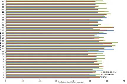
The classification accuracy of the three classification models of SVM CANDEL+SVM CANDEL+ CC-SVM in 30 characteristics of candlestick.
4.
Conclusions
This paper introduces a new forecasting model of financial time series, based on the classification prediction (SVM) model of feature candlestick and cooperative coevolution. characterized Candlestick financial time series reduces the data volume and improves the accuracy of prediction classification. Cooperative coevolution algorithm coordinates three parts in SVM training process, selection of feature subset, number of days window size and selection of optimization algorithm. The cooperative coevolution algorithm and SVM combine to fully consider the relationship between the three components, so that the three components coordinate and work together to achieve higher classification accuracy.
In the experiment, the data came from more than 3,000 stock data, covering the period from 1999 to 2016. Firstly, the data of financial time series with characteristic Candlestick is used to obtain all data that satisfy the particular characteristic Candlestick as the sample point to construct the SVM+CANDEL model. As a comparison, the traditional SVM prediction method was used to randomly select the same number of samples from the same 3,000 stocks as the CANDEL+SVM model. Through training and prediction process, the accuracy of classification prediction was obtained. The classification accuracy of the CANDEL+SVM model is generally higher than the classification prediction accuracy of the simple SVM model. The above comparison experiment verifies the validity of characteristic Candlestick financial time series on its trend prediction. Further, through the Candlestick financial time series, then the SVM combined with CCEA, coordinate the optimal feature subset selection, number of days window size set and optimization algorithm to choose the three parts, establish CANDEL + CC-SVM model, using the same training and testing data sets, to obtain the model prediction accuracy of classification, the characteristic of 30 different Candlestick, CANDEL + CC-SVM model of the classification accuracy is generally higher than the CANDEL + SVM classification prediction accuracy of the model. The above experiments prove that the prediction model of CANDEL+ CC-SVM can effectively improve the prediction accuracy of financial time series compared with traditional methods.
Acknowledgement
Reference
[1] He, J., Tan, A. H., & Tan, C. L. (2003). On machine learning methods for Chinese document categorization.
Applied Intelligence, 18(3), 311-322.
[2] Owusu, E., Zhan, Y., & Mao, Q. R. (2014). An SVM-AdaBoost facial expression recognition system. Applied
Intelligence, 40(3), 536-545.
[3] Hou, C., Nie, F., & Zhang, C. (2014). Multiple rank multi-linear SVM for matrix data classification. Pattern Recognition, 47(1), 454-469.
[4] Castillo, C., Chollett, I., & Klein, E. (2008). Enhanced duckweed detection using bootstrapped SVM
classification on medium resolution RGB MODIS imagery. International Journal of Remote Sensing,
29(19), 5595-5604.
[5] Sirinukunwattana, K., Pluim, J. P., & Chen, H. (2017). Gland segmentation in colon histology images: The
glas challenge contest. Medical Image Analysis, 35, 489-502.
[6] Villarejo, L., Hernando, J., & Padrell, J. (2006). Architecture and dialogue design for a voice operated information system. Applied Intelligence, 24(3), 253-261.
[7] Pons, E., Braun, L. M., & Hunink, M. G. (2016). Natural language processing in radiology: A systematic
review. Radiology, 279(2), 329.
[8] Cambria, E., Xia, Y., & White, B. New avenues in knowledge bases for natural language processing.
Knowledge-Based Systems, 108(C), 1-4.
[9] Zhou, T., Gao, S., & Wang, J. (2016). Financial time series prediction using a dendritic neuron model.
Knowledge-Based Systems, 105(C), 214-224.
[10]Wang, L., & Zhu, J. Financial market forecasting using a two-step kernel learning method for the
support vector regression. Annals of Operations Research, 174(1), 103-120.
[11]He, H., & Starzyk, J. A. (2014). A self-organizing learning array system for power quality classification
based on wavelet transform. IEEE Transactions on Power Delivery, 21(1), 286-295.
[12]Lu, C., Lee, T., & Chiu, C. (2009). Financial time series forecasting using independent component
analysis and support vector regression. Decision Support Systems, 47(2), 115-125.
[13]Lee, K. H., & Jo, G. S. (1999). Expert system for predicting stock market timing using a candlestick chart.
Expert Systems with Applications, 16(4), 357-364.
[14]FISCHER. (1986). Noise. Journal of Finance,41(3), 529-543.
[15]Kim, K. S., Zhao, Y., & Jang, H. (2009). Large-scale pattern growth of graphene films for stretchable
transparent electrodes. Nature, 457(7230), 706-710.
[16]Oliveira, F. B. D., Enayatifar, R., & Sadaei, H. J. (2016). A cooperative coevolutionary algorithm for the
multi-depot vehicle routing problem. Expert Systems with Applications An International Journal,43(C),
117-130.
[17]Yang, Y., He, Z., & Mabu, S. (2012). A cooperative coevolutionary stock trading model using genetic
network programming-Sarsa. Journal of Advanced Computational Intelligence & Intelligent Informatics,
16(5), 581-590.
[18]Rivera, A. J., García-Domingo, B., & Jesus, M. J. D. (2013). Characterization of concentrating photovoltaic
modules by cooperative competitive radial basis function networks. Expert Systems with Applications,
40(5), 1599-1608.
[19]Rabil, B, S., Tliba, S., & Granger, E. (2013). Securing high resolution grayscale facial captures using a
blockwise coevolutionary GA. Expert Systems with Applications An International Journal, 40(17),
6693-6706.
[20]Trunfio, G. A., Topa, P., & Was, J. (2016). A new algorithm for adapting the configuration of
subcomponents in large-scale optimization with cooperative coevolution. Information Sciences, 372,
773-795.
[21]Peng, X., Jin, Y., & Wang, H. Multimodal optimization enhanced cooperative coevolution for large-scale
optimization. IEEE Transactions on Cybernetics, 99.
[22]Sabar, N. R., Abawajy, J., & Yearwood, J. Heterogeneous cooperative co-evolution memetic differential
evolution algorithm for big data optimization problems. IEEE Transactions on Evolutionary
Computation,21(2), 315-327.
[23]Mahdavi, S., Rahnamayan, S., & Shiri, M. E. Cooperative co-evolution with sensitivity analysis-based
budget assignment strategy for large-scale global optimization. Applied Intelligence,47(3), 888-913.
[24]Yang, M., Omidvar, M. N., & Li, C. (2017). Supplementary file of efficient resource allocation in
cooperative co-evolution for large-scale global optimization. IEEE Transactions on Evolutionary
Computation, 99.
[25]Jia, Y. H., Chen, W. N., & Gu, T. (2018). Distributed cooperative co-evolution with adaptive computing
resource allocation for large scale optimization. IEEE Transactions on Evolutionary Computation, 99.
[26]Chandra, R., & Zhang, M. (2015). Competition and collaboration in cooperative coevolution of elman
recurrent neural networks for time-series prediction. IEEE Transactions on Neural Networks &
[27]Gibson, A. K., Stoy, K. S., & Gelarden, I. A. (2016). The evolution of reduced antagonism—A role for host– parasite coevolution. Evolution, 69(11), 2820-2830.
[28]Mei, Y., Omidvar, M. N., & Li, X. (2016). A competitive divide-and-conquer algorithm for unconstrained
large-scale black-box optimization. Acm Transactions on Mathematical Software, 42(2), 13.
[29]Yoder, J. B. (2016). Understanding the coevolutionary dynamics of mutualism with population
genomics. American Journal of Botany,103(10), 1742.
[30]Dorronsoro, B., Danoy, G., & Goire. (2013). Achieving super-linear performance in parallel
multi-objective evolutionary algorithms by means of cooperative coevolution. Computers & Operations
Research, 40(6), 1552-1563.
[31]Malladi, S., Weaver, J. T., & Clouse, T. L. (2011). Moving-average trigger for early detection of rapidly increasing mortality in caged table-egg layers. Avian Diseases, 55(4), 603-610.
[32]Rabiner, L., Sambur, M., & Schmidt, C. Applications of a nonlinear smoothing algorithm to speech processing. IEEE Transactions on Acoustics Speech & Signal Processing, 23(6), 552-557.
[33]Kalman, R. E. (1960). A new approach to linear filtering and prediction problems. Journal of Basic Engineering Transactions, 82, 35-45.
[34]Baraniuk, R. G. (1997). Improved wavelet de-noising via empirical wiener filtering. Proceedings of SPIE
- The International Society for Optical Engineering,3169, 389-399.
Jiang Zhipeng is a graduate student of Information Science and Engineering College of
Shandong Normal University. Following Mr. Luo, he has been studying for more than two years, including data analysis, artificial intelligence and prediction of financial time series. The main interests are artificial intelligence and time series prediction.
Luo Chao is mainly engaged in the theory and application research of evolutionary game,