Advance Access publication 2017 November 6
Modelling the cosmic spectral energy distribution and extragalactic
background light over all time
S. K. Andrews,
1,2‹S. P. Driver,
1,2‹L. J. M. Davies,
1C. d. P. Lagos
1and A. S. G. Robotham
11International Center for Radio Astronomy Research, The University of Western Australia, 35 Stirling Highway, Crawley, WA 6009, Australia 2School of Physics & Astronomy, University of St Andrews, North Haugh, St Andrews KY16 9SS, UK
Accepted 2017 October 31. Received 2017 October 31; in original form 2017 June 13
A B S T R A C T
We present a phenomological model of the cosmic spectral energy distribution (CSED) and the integrated galactic light (IGL) over all cosmic time. This model, based on an earlier model by Driver et al., attributes the cosmic star formation history (CSFH) to two processes – first, chaotic clump accretion and major mergers, resulting in the early-time formation of bulges and secondly, cold gas accretion, resulting in late-time disc formation. Under the assumption of a Universal Chabrier initial mass function, we combine the Bruzual & Charlot stellar libraries, the Charlot & Fall dust attenuation prescription and template spectra for emission by dust and active galactic nuclei to predict the CSED – pre- and post-dust attenuation – and the IGL throughout cosmic time. The phenomological model, as constructed, adopts a number of basic axioms and empirical results and has minimal free parameters. We compare the model output, as well as predictions from the semi-analytic modelGALFORMto recent estimates of the CSED out toz=1. By construction, our empirical model reproduces the full energy output of the Universe from the ultraviolet to the far-infrared extremely well. We use the model to derive predictions of the stellar and dust mass densities, again finding good agreement. We find thatGALFORMpredicts the CSED forz<0.3 in good agreement with the observations. This agreement becomes increasingly poor towardsz=1, when the model CSED is∼50 per cent fainter. The latter is consistent with the model underpredicting the CSFH. As a consequence, GALFORMpredicts a∼30 per cent fainter IGL.
Key words: galaxies: evolution – galaxies: general – cosmic background radiation – cosmology: observations.
1 I N T R O D U C T I O N
One of the goals of modern cosmology is to understand, explain and predict the evolution of mass, energy and structure from the big bang to the present day. Here, we focus on the evolution of energy emanating from the ultraviolet to far-infrared wavelength range – photon production, transport and redistribution – over a 13 billion year timeline (i.e. since recombination). The energy content of the Universe over this wavelength range is often expressed through three measurable quantities: the cosmic spectral energy distribu-tion (CSED) as a funcdistribu-tion of redshift, the extragalactic background light (EBL) and the integrated galactic light (IGL). These quantities are each measurable via distinct direct or indirect methods, but are also closely related. The CSED (e.g. Driver et al.2008; Dom´ınguez et al.2011; Driver et al.2016b; Andrews et al.2017b) describes the
E-mail:[email protected](SKA);[email protected](SPD)
photons generated within a cosmologically representative volume at a specific epoch. The EBL can therefore be expressed as the volume and luminosity distance weighted integral of the redshifted CSED since decoupling. Hence, the EBL describes the distribution of pho-tons observed today, originating from all post-decoupling processes fromλobs=100 nm toλobs=1 mm. The IGL represents the domi-nant component of the EBL and is best derived from number counts of discrete resolved objects (e.g. galaxies and AGN) as observed by a sufficiently deep extragalactic survey (e.g. Driver et al.2016c). In the absence of any diffuse light, the EBL and IGL will be identical – hence, any discrepancy between the two constrains the level of diffuse emission (Driver et al.2016c).
Driver et al.2008, 2016b; Andrews et al. 2017b). The remain-ing photons escape into the intergalactic medium. At higher red-shifts, both components (direct and reprocessed photons) are sup-plemented by mass accretion on to active galactic nuclei (AGN) and their surrounding dust torii (e.g. Richards et al.2006). Again, approximately half of the photons produced by AGN are also at-tenuated. However, in the AGN case the dust torus is significantly hotter and hence re-radiates at mid-infrared wavelengths. Remark-ably, this approximate equality between optical and mid- to far-infrared energy output persists when integrating over all redshifts and is often divided into two distinct components – the cosmic infrared background (CIB, 8 µm< λobs<1 mm in the observed frame; Dwek et al.1998); and the cosmic optical background (COB, 0.1µm< λobs<8µm), see e.g. Driver et al. (2016c).
Given the intimate link between the CSED, the EBL and galaxy evolution, it is insightful to obtain CSED and EBL predictions from semi-analytic (e.g. Gilmore et al.2012; Somerville et al. 2012; Inoue et al.2013) and phenomological models (e.g. Partridge & Pee-bles1967a,b; Finke, Razzaque & Dermer2010; Driver et al.2013; Khaire & Srianand2015) of galaxy formation. Semi-analytic mod-els, e.g. Lacey et al. (2016), begin with dark matter haloes as output from someN-body simulation (e.g. Springel et al.2005), which accrete gas from the intergalactic medium according to a prede-fined prescription. The model determines the star formation his-tory, metallicity evolution and feedback from supernovae and AGN from the accretion rate and the halo merger tree. The unattenu-ated spectral energy distribution (SED) can then be computed using stellar population synthesis codes (e.g. Bruzual & Charlot2003; Maraston2005), with dust attenuation and re-emission added via prescription.
Phenomological models are empirically driven and can be divided into two classes: forward modelling and backward modelling. For-ward models (e.g. Driver et al.2013) are based on measurements or assumptions of
(i) the cosmic star formation history (CSFH; e.g. Hopkins & Beacom2006; Madau & Dickinson2014);
(ii) stellar population synthesis (e.g. Bruzual & Charlot 2003; Maraston2005);
(iii) a known Universal initial mass function (IMF); (iv) the unattenuated SED of starlight; and (v) a dust attenuation and emission model.
Backward modelling arises from evolving observed properties of nearby galaxies, for example luminosity functions (Franceschini, Rodighiero & Vaccari2008) or the classification of galaxies by SED fitting (Dom´ınguez et al.2011), and propagating them backwards in time. Due to their simplistic design and high-level approach, phe-nomological models have fewer free parameters than approaches which look to encode galaxy physics and also recover cluster-ing signatures – i.e. flexible but limited (phenomological) versus comprehensive but immutable (semi-analytic, hydrodynamic and
N-body simulations).
Direct measurements of the COB (e.g. Matsumoto et al.2005,2015; Levenson & Wright2008; Matsuoka et al.2011; H.E.S.S. Collaboration 2013; Biteau & Williams 2015; Ahnen et al.2016; Matsuura et al. 2017; Mattila et al. 2017; Zemcov et al.2017) and CIB (e.g. Puget et al.1996; Fixsen et al. 1998; Hauser et al.1998) have been made using a number of different facilities and methods. Likewise, the IGL has been measured in the ultraviolet and optical (e.g. Madau & Pozzetti2000; Totani et al. 2001; Xu et al. 2005; Keenan et al. 2010) to the mid-and far-infrared (e.g. Dole et al.2006, B´ethermin et al. 2012a;
Carniani et al.2015), with some groups measuring how the CIB accumulates as a function of redshift at specific wavelengths (e.g. Chary & Elbaz2001; Marsden et al.2009; Berta et al.2011; Jauzac et al. 2011; B´ethermin et al. 2012b; Viero et al. 2013). These measurements are usually confined to a single facility and hence a narrow portion of the spectrum.
Robust measurements of the broader CSED have only recently become possible, as they rely on the availability of sufficiently deep and wide multiwavelength data. The first measurement of the dust corrected CSED and hence the far-infrared energy output was made by Driver et al. (2008) from existing optical luminosity den-sity measurements. This measurement was updated by Driver et al. (2012), who integrated luminosity functions from FUV through
Kderived from the Galaxy and Mass Assembly (GAMA) survey. Dom´ınguez et al. (2011) used a SED fitting code in order to interpo-late between broad-band filters, Kelvin et al. (2014) examined the CSED as a function of galaxy morphology and Driver et al. (2016b) extended observations to the far-infrared. Finally, Andrews et al. (2017b) measured the CSED out toz=1 based on a completely homogenous data reduction procedure across the entire ultraviolet to far-infrared wavelength range. In a similar vein, Driver et al. (2016c) computed the extrapolated IGL over the same wavelength range using consistent analysis techniques.
With this data now in hand, this work aims to both extend the Driver et al. (2013) forward model as well as derive a prediction of the CSED and IGL from theGALFORMsemi-analytic model and compare each to the observations. In Section 2, we briefly recap our measurements of the IGL and CSED as reported by Driver et al. (2016c) and Andrews et al. (2017b), respectively. In Section 3, we revisit the Driver et al. (2013) model and extend it to include both dust attenuation and AGN. In Section 4, we derive predictions for both the unattenuated and attenuated CSEDs. In Section 5, we obtain predictions of the CSED from two recent incarnations ofGALFORM. In Section 6, we compute a number of useful relationships from our phenomological model, including the integrated photon escape fraction (IPEF), the comoving IGL and the buildup of dust and stellar mass densities as predicted by our model. We conclude in Section 7.
We use AB magnitudes and assumeH0=70h70km s−1Mpc−1,
=0.7 andm=0.3 throughout.
2 E M P I R I C A L E S T I M AT E S O F T H E I G L A N D C S E D
The genesis of the IGL and CSED data we wish to reproduce is critical to our analysis, so we briefly describe how these data were derived below.
2.1 The integrated galactic light
In Driver et al. (2016c), we measured the IGL from a compendium of deep and wide galaxy number count data from the far-ultraviolet to the far-infrared. This included the GAMA (Wright et al.2016a) and G10/COSMOS (Andrews et al.2017a) data sets as well as a selection of deeper surveys, including data from theGalaxy Evolu-tion Explorer,Hubble,Spitzer,Wide-field Infrared Survey Explorer
in this work. Summing our IGL spectrum over the relevant wave-length ranges, we found values for the COB and CIB of 24±4 and 26 ± 5 nW m−2 sr−1, respectively. These extrapolated IGL measurements agree well with previous literature IGL measure-ments, but fall significantly below the direct EBL estimates based on absolute background analysis of Hubbledata (e.g. Bernstein, Freedman & Madore2002). However, our IGL measurements, with a 20 per cent adjustment upward to account for intrahalo or intra-cluster light and low surface brightness galaxies, agree closely with the high-energy gamma-ray constraints from H.E.S.S. (H.E.S.S. Collaboration2013) and MAGIC (Ahnen et al.2016). Our mea-surements also agree with the direct EBL observations by the Pi-oneer and New Horizons spacecraft taken from the outer Solar system, where the impact of zodiacal light is much less significant (Matsuoka et al.2011; Zemcov et al.2017). This suggests that the direct measurements of the COB may have underestimated the ter-restrial (Earthshine) and/or zodiacal contributions to the total sky background (see e.g. Kawara et al. 2017). In summary, the IGL measurements presented in Driver et al. (2016c) appear robust at all wavelengths with a tentative detection of diffuse light at the 0–20 per cent level in the near-infared.
2.2 The CSED as a function of redshift
While the EBL describes the total integrated light along the path-length of the Universe, the (total) CSED represents its subdivi-sion by redshift. In Andrews et al. (2017b), we measured the (re-solved) CSED from the far-ultraviolet to the far-infrared over a 7.5 Gyr baseline using multiwavelength imagery and spectroscopy from the GAMA (Driver et al. 2011) and COSMOS (Scoville et al.2007) surveys. The GAMA spectroscopic and imaging data are described in Liske et al. (2015) and Driver et al. (2016b) with photometry performed by Wright et al. (2016a), while the assem-bly of redshift and photometric data in the COSMOS region are described by Davies et al. (2015) and Andrews et al. (2017a), respectively.
The photometric measurements were then interpolated using the SED fitting codeMAGPHYS(Multiwavelength Analysis of Galaxy Physical Properties; da Cunha et al.2008) by Driver et al. (2017). As a reminder, theMAGPHYSfits use the Bruzual & Charlot (2003) stellar libraries based on a Chabrier (2003) IMF and the two com-ponent Charlot & Fall (2000) dust attenuation model. The resulting far-infrared dust emission spectrum comprises of polycyclic aro-matic hydrocarbons, warm dust and two populations of cold dust in thermal equilibrium with varying temperatures. The resulting SED fits are generally robust, producing stellar mass and star for-mation rate estimates in line with independent estimates (Taylor et al.2011; Davies et al.2016, see also the direct comparison in Driver et al.2017).
We stacked theMAGPHYSfits for individual galaxies in 10 redshift bins to derive both the unattenuated (dust corrected) and attenuated (observed) CSED for 0.02<z<0.99. We found that the total energy output declined from (5.1±1.0)×1035h
70W Mpc−3atz=0.905 to (1.3±0.3)×1035h
70W Mpc−3at the current epoch, a rate slightly slower than the well-known decline in cosmic star formation (Lilly et al.1996) – as one would expect given that the CSED samples both young and old starlight. The quoted uncertainty in the absolute normalization of the CSEDs ranges from 11 to 27 per cent, and is dominated by cosmic sample variance. Additional, semiquantifiable and wavelength-dependent uncertainties arise from SED modelling error, incompleteness and the lack of complete far-infrared and ultraviolet measurements in G10/COSMOS. These are discussed in Andrews et al. (2017b), their fig. 6 and Section 3.3.
3 R E C O N S T R U C T I N G T H E C S E D
We now look to build a phenomological model of the CSED and elect to follow the pathway laid out in Driver et al. (2013) with the addition of AGN and a more comprehensive dust modelling prescription. To build our revised phenomological model of the energy output of the Universe, one needs:
(i) Empirical estimates of the CSFH (e.g. Hopkins & Beacom
2006; Madau & Dickinson2014; Driver et al.2017).
(ii) The assumption of a mean IMF across cosmic time (e.g. Kennicutt 1983; Kroupa 2001; Baldry & Glazebrook 2003; Chabrier2003).
(iii) A stellar population model (e.g. Bruzual & Charlot2003; Le Borgne et al.2004; Maraston2005).
(iv) A description of how the metallicity of newly formed stars evolves with redshift (Tremonti et al.2004; Erb et al.2006; Zahid, Kewley & Bresolin2011following Driver et al.2013).
(v) A dust attenuation model (e.g. Cardelli, Clayton & Mathis1989; Calzetti et al. 2000; Charlot & Fall 2000; Gordon et al.2003) and corresponding emission spectra in the far-infrared (e.g. Chary & Elbaz2001; Zubko, Dwek & Arendt2004; Draine & Li2007; Dale et al.2014).
(vi) An emission model from AGN (e.g. Elvis et al.1994; Dale et al.2014; Siebenmorgen, Heymann & Efstathiou2015) and either a prescription of linking that to the spheroid star formation rate, or some description of how AGN activity evolves with time (e.g. Richards et al.2006; Palanque-Delabrouille et al.2016).
Constructing a model in this manner should, in theory, require no tunable initial conditions – the choice of parameters in stellar, dust and AGN modelling should all be guided by empirical data. However, free parameters are unavoidable when the available data are insufficient to constrain the model. At the heart of the Driver et al. (2013) two-phase model there are two axioms, which we also adopt here:
(i) AGN activity traces stellar mass growth in spheroids. (ii) The formation of material ending up in spheroids today dom-inates at high redshift.
The first axiom is based on the Mbh–M∗, sph and Mbh–σ rela-tions (Magorrian et al.1998; Gebhardt et al.2000), which implies co-evolution between the central black hole and the surrounding spheroid (Silk & Rees1998; Kormendy & Ho2013; Graham & Scott2015). However, while theMbh–M∗, sphrelation is irrefutable, multiple studies have found no or only weak correlation between total (i.e. disc and spheroid) star formation and AGN activity (Mul-laney et al. 2012a; Rosario et al. 2012; Stanley et al.2015). At
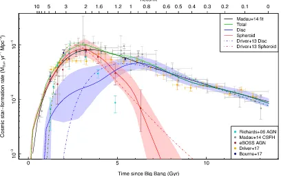
Figure 1. Our fitting functions to the CSFH for discs (blue), spheroids (red) and combined (green) compared to those for Driver et al. (2013) (dashed line) and Madau & Dickinson (2014) (solid black line). The corresponding error regions in the disc and spheroid CSFHs are also shown. The Madau & Dickinson (2014) CSFH data (grey points), the Driver et al. (2017) and Bourne et al. (2017) CSFH data (orange and dark blue points, respectively) and the Richards et al. (2006) AGN luminosity function data scaled to the Madau & Dickinson (2014) fitting function (red points) are also shown.
The case for the second axiom is stronger. The recent advent of integral field spectroscopic observations has enabled more robust determination of the mass growth history of galaxies. McDermid et al. (2015) found that early-type galaxies have formed 50 per cent of their stars byz=3 and 90 per cent byz∼0.9. A similar picture is painted by Ibarra-Medel et al. (2016), with red, quiescent, high-mass and/or early-type galaxies forming a greater portion of their stars at higher redshifts. In both studies, low-mass galaxies undergo steady mass growth to the current epoch. Gonz´alez Delgado et al. (2015) showed that early-type galaxies contain older stellar populations (log (age)∼9.5–10) than late-type galaxies (log (age)∼8.5–9.5). Sa and Sb types show an older stellar population at low galactocen-tric radii, potentially corresponding to bulge material. Early-type and high-mass galaxies contain the majority of spheroid material in the Universe, while low-mass galaxies consist of predominantly disc material (e.g. Moffett et al.2016a). This is consistent with the scenario we envisage in the two-phase model – spheroid star for-mation occurring primarily at higher redshifts, while star forfor-mation linked to cold gas accretion continues in low-mass galaxies and discs to the current epoch.
We proceed under the assumption that AGN activity is causally linked to, or coincidental with spheroid star formation on a time-averaged basis and now build up our model over five key stages:
(i) Compute the unattenuated CSED from the CSFH and an adopted gas-phase metallicity evolution.
(ii) Compute the attenuated CSED from a set of selected dust attenuation parameters, given the CSFH and metallicity evolution in stage 1.
(iii) Add far-infrared spectra based on the attenuated energy de-rived in stage 2.
(iv) Add AGN spectra based on the evolution of the AGN lumi-nosity function with redshift.
(v) Construct the IGL from the full CSED as a function of red-shift.
These ingredients are described below.
3.1 The cosmic star formation history
We take the opportunity to update the Driver et al. (2013) fitting functions of the CSFH as follows:
We replace the compilation of cosmic star formation rate mea-surements with that from Madau & Dickinson (2014) augmented by the recent measurements from Driver et al. (2017) and Bourne et al. (2017). We replace the Richards et al. (2006) AGNi-band total lumi-nosity data withg-band (rest frame) data from the extended Baryon Oscillation Spectroscopic Survey (eBOSS; Palanque-Delabrouille et al.2016). We calculated the total quasar luminosity and error from the 16th, 50th and 84th percentile of 1000 Monte Carlo inte-grations of the pure luminosity-evolution model of the Palanque-Delabrouille et al. (2016) quasar luminosity function.
We scale the peak of the eBOSS total quasar luminosity, which occurs atz=2.01, to the Madau & Dickinson (2014) fitting function. From this, we determine the CSFH for spheroids by fitting an eight-point spline weighted by the inverse relative error squared using the compiled CSFH data forz>2.01 and the eBOSS AGN data below this redshift (red line on Fig.1). We elect to use the compiled CSFH data above the peak redshift because it is more comprehensive and precise than the AGN data – in the adopted model, about half of spheroid stellar mass forms prior toz=2.01.
model, an obscured fraction which evolves with redshift changes how quickly spheroid star formation activity declines sincez∼2 if we maintain that the spheroid CSFH is equal to the total CSFH prior to that redshift. The evolution of the obscured AGN fraction as a function of redshift is still unclear. Treister & Urry (2006) find from quasar X-ray luminosity functions that the obscured frac-tion evolves as (1+z)0.3–0.4, while Lusso et al. (2013), also using X-ray data, find no evidence for evolution. The shape of the spheroid CSFH has direct consequences for the bulge to disc stellar mass ra-tio, and corresponding CSEDs, atz= 0. Adopting the evolution in Treister & Urry (2006) will result in a steeper drop-off in the spheroid CSFH, less spheroid stellar mass and a fainter spheroid CSED atz=0. Conversely, adopting an X-ray luminosity density evolution that declines more slowly, as in, e.g. Ueda et al. (2014) re-sults in the opposite. Similarly, adopting an earlier (later) peak will result in less (more) spheroid stellar mass and redder, fainter (bluer, brighter) emission atz=0. Accurate bulge-disc decomposition over the 0.1<z<2 range, and corresponding stellar mass estimates, will test these scenarios and allow the reconstruction of the disc and spheroid CSFHs without the need to adopt AGN activity as a proxy. The CSFH for discs (solid blue curve in Fig.1) is determined by fitting an eight point spline to the Madau & Dickinson (2014) CSFH data minus the CSFH for spheroids. Each spline is then extrapolated to cover lookback times between 0 and 13.5 Gyr. We also impose a CSFH floor of 10−4M
yr−1Mpc−3to reduce the numerical integration error arising when deriving the stellar mass density in spheroids.
The resulting CSFH functions and data are shown in Fig. 1. The transition from spheroid star formation to disc star formation happens∼1 Gyr later (z∼1.2 compared toz∼1.7) in this model compared to Driver et al. (2013). This is due to the use of the eBOSS AGN data, and a higher CSFH for spheroids at very high redshift because we fit to the CSFH data instead of the AGN data. Combined with using spline fitting to avoid assuming a functional form, this improves the fitting of the CSFH at high redshifts over the Driver et al. (2013) model. The precise shape of the disc CSFH att∼5 Gyr is, to some degree, a byproduct of the spline fitting and subtraction and has little physical significance. Otherwise, the fitting functions are similar to those adopted by Driver et al. (2013) for the CSFH for spheroids and discs (dashed lines).
We estimate the error associated with the CSFH by repeating the spline fitting procedure for the lower and upper bounds of the individual CSFH data points and show the error regions on Fig.1. The resulting≈40 per cent error in the total CSFH atz=0 represents a conservative estimate of the error in the CSFH by itself. It is more reasonable as an estimate of total model error, which incorporates uncertainties in the model assumptions, the IMF, stellar libraries and gas phase metallicity.
3.2 Model stellar populations
[image:5.595.308.542.61.289.2]To model the stellar population, we use theGALAXEVsoftware and the Bruzual & Charlot (2003) stellar models for consistency with the Andrews et al. (2017b) empirical CSED measurement. Both the Bruzual & Charlot (2003) andPEGASE2 (Le Borgne et al.2004) model used by Driver et al. (2013) employ the same set of Padova (1994) isochrones, but differ in their underlying library of stellar atmospheres – Bruzual & Charlot (2003) uses the theoretical BaSeL library (Allard & Hauschildt1995) whilePEGASE2 uses the empir-ical ELODIE library (Prugniel & Soubiran2001). The difference between the two stellar libraries should be small over the relevant wavelength range (Conroy & Gunn2010). A detailed exploration of
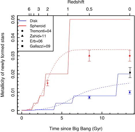
Figure 2. The adopted metallicity of newly formed stars for spheroids (red) and discs (blue). Metallicity curves in the absence of rounding are shown in dashed lines. The inferred metallicities of spheroids and discs, from Driver et al. (2013) based on the underlying Tremonti et al. (2004), Erb et al. (2006) and Zahid et al. (2011) data, as well as the cosmic stellar phase metallicity (Gallazzi et al.2009) are also shown.
the effect of assuming different stellar libraries on the empirical and model CSEDs would require refitting SEDs to subsamples of the Driver et al. (2017) catalogue and is outside the scope of this paper. Regardless, any differences are not likely to be significant in light of measurement and other model uncertainties. If the BC03 libraries are found to be insufficiently accurate, the CSED measurements and models will need to be revised accordingly.
We use a Chabrier (2003) IMF, again to be consistent with the empirical CSED measurement. [The Driver et al. (2013) model uses a Baldry & Glazebrook (2003) IMF, which can be converted to a Chabrier IMF by scaling the CSFH appropriately.]
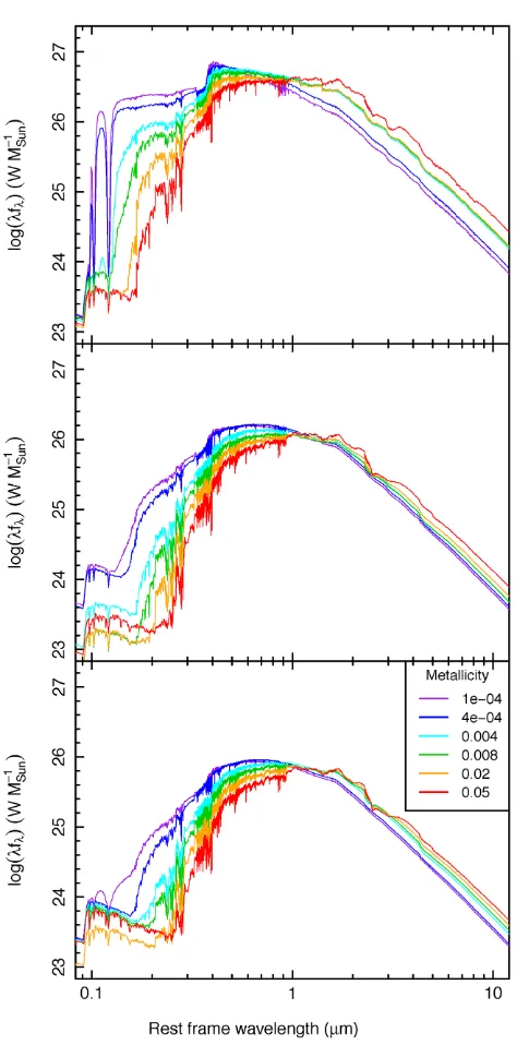
Figure 3. Unattenuated SEDs for simple stellar populations constructed using the CSFH for discs 8 Gyr after the big bang with the indicated metal-licities at an age of 1 Gyr (top), 5 Gyr (centre) and 10 Gyr (bottom). The units on theY-axis are watts per solar mass of stars formed.
For illustration purposes, Fig.3shows SEDs for simple stellar populations with ages 1, 5 and 10 Gyr as a function of metallicity. The input CSFH is that for discs at 8 Gyr after the big bang. While the model CSEDs vary considerably in the ultraviolet and short-wavelength optical, the total flux output varies by only 0.3 dex in the near-infrared between the most extreme metallicities. The least scatter occurs in the rest-frameYband – at 1µm, flux ranges from 1026.44 W per solar mass of stars formed (Z= 0.0001) to 1026.64 W M−1
(Z=0.004) att=1 Gyr. The spread decreases to between 1026.07 W M−1
(Z=0.0004) to 1026.14 W M−1
(Z=0.008) att= 5Gyr and 1025.82 W M−1
(Z =0.004) to 1025.91 W M−1 (Z=0.05) att=10 Gyr.
From our adopted CSFH, IMF and metallicity evolution, 61 and 74 per cent of stellar mass forms at metallicities between 0.004 and 0.02 for both spheroids and discs, where the near-infrared flux difference is negligible. Imprecision in modelling metallicities may affect the blue portion of the spheroid CSED notably, but the impact on the overall CSED is minimal.
3.3 Dust modelling
To model dust attenuation we use the Charlot & Fall (2000) extinc-tion model built in toGALAXEV. We set theV-band optical depth (τV) as seen by stars in birth clouds to
τV(t)a=Xexp
−t
2.5
t
0
0.004 csfh(t) exp
t
2.5
dt, (1)
wheretandtare ages of the Universe in Gyr,Xis the normalization constant necessary to yieldτV(13.5 Gyr)=1.2 for discs and 0.25 for spheroids, csfh(t) is the CSFH for spheroids or discs anda=
2 for discs and 1/0.65 for spheroids. The right-hand side of theτV model is the dust mass density evolution from Driver et al. (2017). This model is based on measurements of the dust mass density by M´enard & Fukugita (2012) and B´ethermin et al. (2014), and predicts that 0.4 per cent of mass forming into stars returns to the ISM as dust, with an exponential destruction with a characteristic time of 2.5 Gyr (see Driver et al.2017for details). We choose the model involving exponential dust destruction – the alternative model where some fraction of dust survives indefinitely is inconsistent with elliptical galaxies being largely dust free atz=0. The values ofτV(13.5 Gyr) are chosen to yield a time evolution consistent with the median
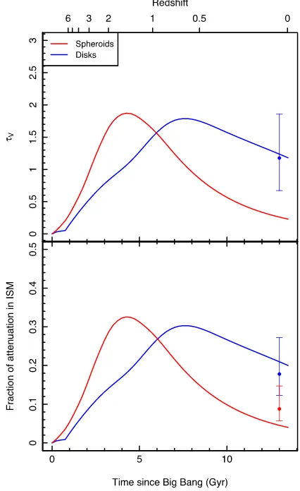
τV(13.5 Gyr) value from the Driver et al. (2017) fits. We apply a similar prescription to the fraction of attenuation arising in the ISMμ, settingμ(13.5 Gyr) to be 20 and 4 per cent for discs and spheroids, respectively. The chosen values forμare guided by the medianμ(z<0.06) derived from spheroid and disc samples created by matching against the GAMA VisualMorphologyv03 catalogue1 Ultimately, the values ofτV(13.5 Gyr), μ(13.5 Gyr) and the free parameterafor discs are chosen to reproduce the ultraviolet, post-attenuation CSED for 0< z< 1 (especially at lower redshifts). The corresponding values regarding spheroids are less certain, but are chosen such that the resulting ultraviolet extinction is consistent with the empirical data. These functions and estimates are shown in Fig.4. The error bars shown represent the 16th and 84th percentile of the distribution as an indication only; we acknowledge that our empirically derived dust attenuation parameters are subject to large SED modelling errors due to limited sensitivity in the far-infrared at the current time.
We model the far-infrared emission with models from Dale et al. (2014) scaled up to the total energy attenuated. Dale et al. (2014) model the emission from dust exposed to 64 different heat-ing intensities as described by the parameterαsf, where model 1 (αsf=0.0625) has the most heating and model 64 (αsf=4.0000) the least. These models improve on the Dale & Helou (2002) models used by Driver et al. (2013) by updating the mid-infrared observa-tions on which the models are based and adding in emission from the dust torii of AGN. The main difference between these models and those used byMAGPHYSin the Andrews et al. (2017b) empirical
1The spheroid value was derived from an elliptical sample defined by
[image:6.595.48.285.48.527.2]Figure 4. The adoptedτV (top) andμ(bottom) for spheroids (red) and
discs (blue).
CSED estimates is that the Dale et al. (2014) models produce less 70µm emission. This difference is immaterial given the lack of constraining data near this wavelength. As the Dale et al. (2014) templates are in arbitrary units, we scale to reflect the total attenu-ated energy implied by our stellar model and equation (1) (integrattenu-ated over 10 nm< λ <8µm).
Initially we select the set of models with a zero AGN fraction. At all redshifts, we assume 15 per cent of the far-infrared radiation emitted originates from galaxies with warmer dust temperatures (such as ultra-luminous infrared galaxies) and 85 per cent from the broader infrared galaxy population. This assumption is reason-able, given>90 per cent of the normal infrared galaxy population and>60 per cent of the luminous infrared galaxy population have dust temperatures<35 K out toz=0.5 (Symeonidis et al.2013). This ratio is slightly lower than the 25 per cent contribution from ultra-luminous infrared galaxies to the IGL at 140µm modelled by Chary & Elbaz (2001), however we find the lower ratio represents a better fit to the Andrews et al. (2017b) attenuated CSEDs. This is not definitive, given that the photometry underlying the Andrews et al. (2017b) far-infrared CSEDs is of relatively low depth and sensitivity; this also prevents computation of robust total infrared luminosity functions.
We select model 33 (αsf=2.0625) and 37 (αsf=2.3125) for in-frared luminous and normal galaxy populations respectively atz=0,
the combination of which reproduces the Andrews et al. (2017b) far-infrared CSED between 100 and 500µm forz<0.14 well. At higher redshifts, we evolve the luminous galaxy model selection by select-ing αsf = 1.3750+ 0.6875 log(CSFH(13.5 Gyr))/log(CSFH(t)), withαsffor normal galaxies being 0.500 greater than that for in-frared luminous galaxies. This evolves the dust emission spectra towards a higher temperature on average – from 25–32 K atz=0 to 32–41 K at the peak of star formation atz∼2 – in accordance with increased far-infrared emission and theLir–Tdustrelation (Symeoni-dis et al.2013). These dust temperatures are also consistent with those observed by Symeonidis et al. (2013) over this redshift range. A weak dependence on the CSFH is also expected as increased heating from a higher CSFH is partially offset by increased dust masses, as noted by Symeonidis et al. (2013) and Driver et al. (2017). This particular selection appears to reproduce the Andrews et al. (2017b) far-infared CSED well, however we caution that this estimate is based on a significant fraction of extrapolated flux. Fur-thermore, the Symeonidis et al. (2013) data probe galaxies with
Lir >1010L increasing to 1011.8Latz =1, and the normal infrared galaxy population out toz=0.3, representing an incom-plete picture of dust temperatures across the galaxy population out toz=1.
3.4 AGN modelling
We represent emission from AGN in two classes – obscured and unobscured. We derive an unobscured AGN composite spectrum from the sum of the SDSS composite quasar spectrum published by vanden Berk et al. (2001) and the 100 per cent AGN fraction Dale et al. (2014) model. To obtained an obscured AGN spectrum, we multiply the quasar composite spectrum by the IPEF as measured by Andrews et al. (2017b) for 0.82<z<0.99 to represent dust attenuation and add the hottest Dale et al. (2014) model (number 1) to represent attenuation of AGN emission in the broader ISM. We scale the obscured and unobscured AGN spectra to yield ag-band rest-frame luminosity equal to 2 and 1 times the eBOSS integrated
g-band luminosity of Palanque-Delabrouille et al. (2016) respec-tively (the Palanque-Delabrouille et al.2016data trace the evolu-tion of unobscured AGN) for an obscured to total AGN emission ratio of 67 per cent. Observations indicate a ratio of obscured to total AGN emission ranging between 41 and 77 per cent, with the majority of estimates towards the upper end (Richards et al.2006; Buchner et al.2015). This ignores the evolutionary biases traced by AGN (e.g. being more common in dust-free early-type galaxies), but the impact of this assumption should be limited by the high photon escape fractions for these systems. AGN host galaxies were not included in the Driver et al. (2017) fits, and do not represent a significant addition to the Andrews et al. (2017b) CSED at any
z<0.99 – Andrews et al. (2017b) find an extra 5–10 per cent con-tribution to the CSED from X-ray emitting AGN and their host galaxies except possibly in the ultraviolet as noted by Driver et al. (2016c).
4 M O D E L O U T P U T S
4.1 The unattenuated CSED
Fig.5shows the predicted unattenuated CSED int(rest frame, in
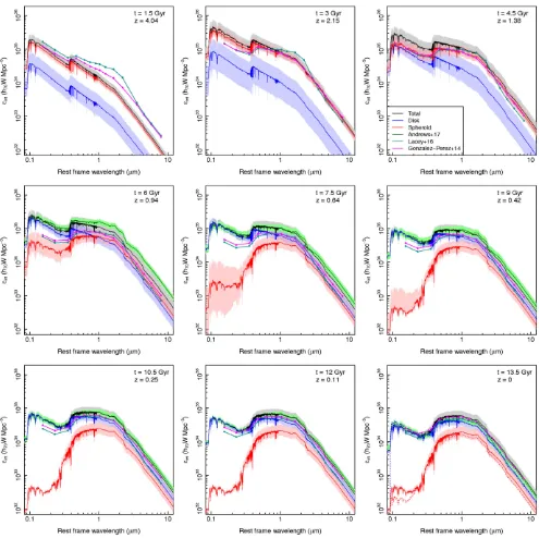
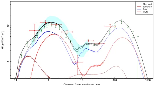
Figure 5. The model unattenuated CSED for spheroids (red), discs (blue) and both combined (black), with shaded areas representing model uncertainty. The Andrews et al. (2017b) data are also given (green line/band), with the uncertainty range indicating the error in the normalization of the CSED only. We also extrapolate this data toz=0. Semi-analytic predictions fromGALFORMare shown in dark cyan (Lacey et al.2016) and pink (Gonzalez-Perez et al.2014). An animated version of this figure is available online as supporting information.
While not shown in the figure (as the data probe a period between 12.2 and 13.3 Gyr), the Driver et al. (2012) model lies within, but close to the lower bound of the uncertainty range of the CSED measurement. We also extrapolate the Andrews et al. (2017b) CSED estimates toz=0 by rescaling the 0.02<z<0.08 CSED by the expected decline in total integrated energy. The error range depicted in Fig.5for the Andrews et al. (2017b) data represents the error in the normalization of the CSED only and does not incorporate any contribution from errors in SED modelling, incompleteness or photometry.
From Fig.5, we can extract a number of key conclusions. The changeover from major mergers (spheroid formation) to cold gas accretion (disc formation) – where emission from discs dominates in the rest-frame ultraviolet – occurs atz∼1.2, in line with the CSFH (see Fig.1). Cold gas accretion primarily occurs in low-mass (M∗<∼5×10¹⁰M
for a 0<z<0.5 GAMA sample) galaxies, with merger accretion continuing in high-mass galaxies (Robotham et al.2014). The total energy output of the Universe reaches a maximum of 5.0+−21..76×1035
W Mpc−3atz≈0.8. To date, just above half (50.6 per cent) of the energy generated by the Universe was generated by objects now residing in discs, with the other half being generated by material now residing in spheroids. For reference, 50 per cent of the stellar mass today resides in spheroids, with the other 50 per cent in discs (Moffett et al.2016b).
Recall that the model is calibrated on the CSFH, and therefore is designed to reproduce the (unattenuated) ultraviolet emission. How-ever, the Andrews et al. (2017b) empirical CSEDs have a number of caveats which may become reflected in the model. First, the empiri-cal CSEDs may suffer from incompleteness due to Malmquist bias, resulting in the omission of low-mass, blue, star-forming systems. Andrews et al. (2017b) estimate that this incompleteness causes of the order of 20 per cent of the ultraviolet flux to be missed. Sec-ondly, the Wright et al. (2016a) catalogue, on which the empirical CSEDs are based, measures ultraviolet flux in an optically defined aperture convolved with the GALEXpoint spread function. This approach may miss additional, extended ultraviolet emission from disc galaxies (Gil de Paz et al.2005; Thilker et al.2007) forz<0.45. Our model reproduces the unattenuated CSED in the near-infrared well, except arguably atz∼ 0.9, where we see a slight deficit in the model. Uncertainties in the near-infrared may be the result of a number of factors:
(i) Uncertainties in modelling thermally pulsating asymptotic gi-ant branch stars. We have tried to control for this effect, as both the phenomological model and CSED estimates are based on the Bruzual & Charlot (2003) stellar libraries.
(ii) Uncertainties and imprecisions in modelling gas-phase metallicity. However, Fig.3shows these have a much greater effect in the ultraviolet and optical shortward of the 4000 Å break and opposite effects either side of about 1µm. This would suggest that the lack of metallicity interpolation is not the dominant source of modelling error.
(iii) The photometric and spectroscopic data underlying the Andrews et al. (2017b) measurements use an observed frame
r- ori+-band selection. At the high-redshift ends of GAMA and G10/COSMOS, this is equivalent to uor gin the rest frame. It is, hence, likely that some quiescent or very dusty galaxies are excluded.
(iv) The Driver et al. (2013) model applies a 25 per cent down-ward adjustment to the CSFH for spheroids, resulting in a spheroid to disc mass ratio at the current epoch of∼2
3. This renormalization is not necessary in our model – see Section 6.4.
Overall, our phenomological model appears to reproduce the Andrews et al. (2017b) unattenuated CSED forz<1 extremely well. The black model line lies close to, or within the green measurement band (which takes into account uncertainty in the normalization of the CSED only, excluding the biases noted above and in Andrews et al. 2017b) at all redshifts – with just a minor discrepancy in the near-infrared CSED in the 0.82 < z< 0.99 bin. The model uncertainty at optical wavelengths and low redshifts is mostly due to uncertainty in the CSFH at high redshifts. An animated version of Fig.5is available online as supporting information.
4.2 The attenuated CSED
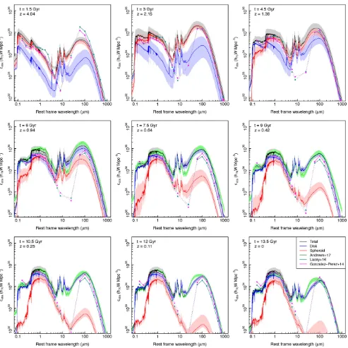
We now add in our dust prescription as described in Section 3.3 to determine the attenuated (as observed) CSEDs. Fig.6shows the resulting attenuated CSED obs, now with far-infrared emission at various time-steps with the Andrews et al. (2017b) attenuated CSED data at the relevant time-steps. The Andrews et al. (2017b) data have
been extrapolated toz=0. The Driver et al. (2012) model, being relevant for 0.013<z<0.1 and thus not shown above, generally lies within the uncertainty range of the empirical CSED estimates. Again, the error range in the empirical CSEDs reflects the error in the normalization of the CSED only, excluding uncertainties in SED modelling and the underlying photometry.
Both optical and far-infrared emission reach a maximum of 2.2+−10..48and 3.7−1.71.1×1035h70 W Mpc−3atz≈2.1.
The most noticeable disagreement between the phenomological model and the CSED data occurs at around 70µm. Empirically,
MAGPHYSis unable to constrain the warm dust peak resulting from
the lack of sufficiently deep 70µm data in both the GAMA and G10/COSMOS data sets. The choice of different dust emission templates to model the far-infrared emission is also important – Driver et al. (2012) use the average of Dale & Helou (2002) models 34 and 40, which results in a small warm dust peak that is slightly below our model curve. Ultimately, the far-infrared imaging data underlying the SED fits is of poorer quality in terms of resolution and sensitivity – the CSED estimates are only precise to a factor of about 2 at low redshifts, increasing to a factor of 5 beyond
z=0.45. Estimates in G10/COSMOS are based on a significant fraction of extrapolated flux, while in GAMA the low detection rate undermines the reliability of the corresponding CSED (see fig. 7 in Andrews et al.2017b). We denote wavelength intervals where the CSED estimates may be unreliable with a dashed (as opposed to solid) line. For this reason, a rigorous optimization against the Andrews et al. (2017b) CSED estimates between 100 and 500µm is not possible.
Otherwise, our phenomological model again reproduces the at-tenuated CSED well at all redshifts – lying within or close to the green error bounds of the normalization of the CSED only (which excludes SED modelling error, incompleteness and bias) with two exceptions, the first being thez∼0.91 shortfall in the near-infrared mentioned previously. Secondly, the model overpredicts flux at 20µm. This is a consequence of differing prescriptions of warm dust used by the empirical CSED measurements and the model pre-dictions, coupled with the difficulty of correctly modelling emission from polycyclic aromatic hydrocarbons and the incompleteness of the observational data at this wavelength. An animated version of Fig.6is available online as supporting information.
5 S E M I - A N A LY T I C M O D E L L I N G W I T H G A L F O R M
The phenomological model described in Section 3 is a simplistic description built explicitly to model the CSED, providing an in-stant CSED prediction at any redshift to help interpret the EBL and photon escape fraction (see below). While it has predictive power outside this domain – one can infer the cosmic stellar and dust mass densities – many phenomena are neglected (for exam-ple, variations with environment). Semi-analytic models are able to provide a broader understanding, but at the expense of additional complexity.
Figure 6. The model attenuated CSED with labelling equivalent to Fig.5. Wavelength intervals where the Andrews et al. (2017b) CSEDs may be deemed less reliable due to the lack of underlying photometric data and where semi-analytic predictions fromGALFORMomit flux from warm dust are denoted with a dotted line. An animated version of this figure is available online as supporting information.
250, 350, 500, 850 and 870µm. We then multiply by the respec-tive luminosities and sum to arrive at the corresponding luminosity density for each band. The resulting predicted (rest frame) unat-tenuated and atunat-tenuated CSEDs are shown in Figs5and6, respec-tively – the Lacey et al. (2016) is denoted with dark cyan curves, while the Gonzalez-Perez et al. (2014) model is denoted with pink curves.
The twoGALFORMflavours presented here were calibrated to fit theBj- andK-band luminosity functions atz=0, and the evolution of theK-band luminosity function out toz∼ 3. In addition, the Lacey et al. (2016) model paid close attention to number counts and redshift distributions of sources observed byHerscheland at
850µm. Therefore, the comparisons we derive here (i.e. the IGL and evolution of the CSED) are mostly independent tests that can offer valuable insight into how the models can be improved.
– for spheroid star formation. In contrast, the Gonzalez-Perez et al. (2014) version assumes a Universal Kennicutt (1983) IMF.GALFORM predicts an earlier transition from spheroid to disc formation than the phenomological model –z∼3 compared toz∼1.2 (see Lacey et al.2016, fig. 26).
Mock photometry is computed in the Lacey et al. (2016) model using the Maraston (2005) stellar population synthesis codes, while the Gonzalez-Perez et al. (2014) model uses the Bruzual & Charlot (2003) libraries. The Maraston (2005) libraries track fuel consumption, in contrast to the isochrone analysis em-ployed by Bruzual & Charlot. The modelling of thermally pulsat-ing asymptotic giant branch stars is still controversial, with the Maraston libraries arguably overestimating the near-infrared emis-sion (see e.g. Maraston2005; Maraston et al.2006; Bruzual2007; Conroy & Gunn 2010; Bruzual et al. 2013; No¨el et al. 2013; Capozzi et al.2016). The use of the Maraston stellar libraries is the most likely cause of the near-infrared enhancement of the Lacey et al. (2016) model over both the phenomological model and the Gonzalez-Perez et al. (2014) model atz>1 in both the unattenuated and attenuated CSEDs (see Figs5and6).
GALFORMcan also compute dust attenuation via radiative transfer through a two-phase medium consisting of molecular clouds and the diffuse ISM, with dust emission described using a modified blackbody spectrum (Lacey et al.2016).GALFORMdoes not model the mid-infrared emission as it does not incorporate polycyclic aromatic hydrocarbons (Cowley et al.2017). As a consequence, the predicted attenuated CSED is unreliable between 8 and 70µm rest frame. This region is denoted with a dotted line in Fig.6.
BothGALFORMmodels underpredict the CSFH forz<3 (Mitchell et al.2014; Guo et al.2016; Lacey et al.2016) compared to literature estimates (e.g. Madau & Dickinson2014). The predictions, how-ever, agree with the lower CSFH derived by Driver et al. (2017) (on which the empirical CSED estimates are based). However,GALFORM produces a fainter unattenuated CSED than our empirical results. When adjusted for this offset, both semi-analytic models produce a shape of the unattenuated CSED that is very similar to our CSED estimates. Beyondz = 3, theGALFORM predictions of the CSFH show a better agreement with observations. Far-infrared emission grows faster than optical emission in both iterations ofGALFORMat very high redshifts. This originates from obscured star formation in ultra-luminous infrared galaxies, which contribute a much greater portion of the total far-infrared luminosity at higher redshifts (Lagos et al.2014). This effect is not accounted for in the phenomological model.
When adjusted for the offset in the CSED normalization, both GALFORMmodels reproduce the shape of the optical and near-infrared attenuated CSED well out toz=1 (Fig.6). Na¨ıvely, the Gonzalez-Perez et al. (2014) model yields a better fit in the far-infrared. How-ever, when adjusted, both models overpredict the ultraviolet CSED, with the Lacey et al. (2016) model being closer to the empirical data. We suspect the underpredicted dust attenuation is a result of overpredicted galaxy sizes – Merson et al. (2016) show thatGALFORM is able to derive reasonable predictions for dust attenuation when the predicted half-mass radii are also plausible. However, galaxies with overpredicted sizes have much less attenuation than expected, as the diffuse dust component has a lower surface density.
In summary, both iterations ofGALFORMunderpredict the CSFH forz<3 and thus the normalization of the unattenuated and at-tenuated CSEDs. Both semi-analytic models are able to reproduce the shape of the unattenuated and attenuated CSEDs well out to
z<1, with the exception that both models seem to underpredict the ultraviolet attenuation over 0<z<1. In the absence of higher
redshift CSED estimates, we look to constraints on the EBL, COB and CIB.
6 A P P L I C AT I O N O F T H E M O D E L
Having developed a model which replicates the unattenuated and attenuated CSEDs forz< 1, we can now explore predictions of related quantities, such as the photon escape fraction, IGL, and stellar and dust mass densities compared to observations.
6.1 The integrated photon escape fraction
The IPEF represents the attenuated CSED divided by the unattenu-ated CSED. It is a simplistic but useful representation of the effects of dust attenuation. It is particularly useful for correcting ionizing radiation pervading the ISM and/or determining unattenuated star formation rates. The predominant source of error in the IPEF arises from SED modelling and incompleteness – the uncertain normal-ization due to cosmic variance, sampling and the use of photometric redshifts is divided out. The uncertainty arising from the CSFH also cancels.
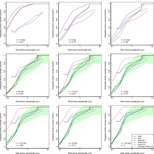
Fig.7shows IPEFs as a function of redshift for both our model (smoothed with a spline interpolation) and the Andrews et al. (2017b) data (green shaded band). The disc IPEF reproduces the Andrews et al. (2017b) IPEFs well, especially at lower redshifts. The overall IPEF reaches a minimum longwards ofλ=700 nm atz∼1.7. The ultraviolet IPEF has two minima – one atz≈1.7, the other atz≈0.6. Spheroids become more transparent than discs across the electromagnetic spectrum atz∼0.9. Our methodology assumes dust emission is negligible. The spike in the photon es-cape fraction at approximately 3µm is a consequence of the 3.3µm polycyclic aromatic hydrocarbon emission feature and should not be regarded as an estimate of the photon escape fraction at that wavelength.
As noted before and in Gonzalez-Perez et al. (2017), both iter-ations ofGALFORMunderpredict the amount of dust attenuation for
z<1 compared to the Andrews et al. (2017b) empirical CSED es-timates. The lack of a prescription for warm dust is the most likely cause for the shortfall in the mid-infrared.
One commonly used method to measure the CSFH involves de-termining the rest-frame far-ultraviolet luminosity function and correcting it for attenuation (see e.g. Kennicutt1998; Madau & Dickinson 2014), usually using either the Calzetti et al. (2000) law or the IRX (=Lir/LFUV)–β relation (Meurer, Heckman & Calzetti1999). For the latter,AFUVcan be computed directly from IRX. Here, we simply computeAFUVby convolving the IPEF with theGALEXFUV filter curve and converting to magnitudes. Fig.8
shows predictions ofAFUV compared to the empirical data from Cucciati et al. (2012), Burgarella et al. (2013) and Andrews et al. (2017b). The phenomological model obtains predictions ofAFUV that are broadly consistent with the empirical data at most red-shifts, whileGALFORMgenerally underpredictsAFUV. Atz∼4, the phenomological model appears to predict a lowerAFUV than the literature. However, at these redshifts, dust attenuation starts to de-viate from the IRX–βrelation (Capak et al.2015). These redshifts are beyond the scope of this paper.
6.2 The integrated galactic light
Figure 7. The model IPEF for spheroids (red), discs (blue) and both combined (black) with semi-analytic predictions fromGALFORM(dark cyan, pink). The
Andrews et al. (2017b) data are also given in green.
Gilmore et al. (2012) predictions from the semi-analytic model of Somerville et al. (2008) and Somerville et al. (2012). In short, this model uses a Chabrier (2003) IMF, the Bruzual & Charlot (2003) stellar libraries, a modified Charlot & Fall (2000) dust attenuation model and far-infrared spectra from Rieke et al. (2009), which are derived from (ultra)-luminous infrared and low-redshift galaxies.
The comoving EBL at redshiftzis the amount of radiation re-ceived by an observer at a given epoch and may be derived from the (total) CSED as follows:
EBL(λobs, z)=
z=∞
z=z
(λ(1+z), z)dV(z)
4πdl(z)2 , (2)
where (λ,z) is the rest-frame attenuated CSED at the redshiftz,
dl(z) is the luminosity distance atzto the volume corresponding to the redshiftzand dV(z) is the differential comoving volume of each model time-step subtending a solid angle of 1 sr.
Figure 8. Rest-frameAFUVas a function of redshift from the
phenomo-logical model (blue: disc, red: spheroids, black: weighted average by the cosmic star formation rate in each component),GALFORM, the Andrews et al. (2017b) estimates, Cucciati et al. (2012) and Burgarella et al. (2013).
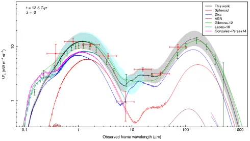
observations are able to constrain the amplitude of the COB, but draw upon the Franceschini, Rodighiero & Vaccari (2008) and Dom´ınguez et al. (2011) models, respectively, to define the shape. The red points representγ-ray observations from Biteau & Williams (2015), which do not assume an EBL model spectrum.
As expected, emission from low-redshift discs dominates at ultra-violet, optical and far-infrared wavelengths. Longwards of 350µm, we find that high-redshift spheroids represent the dominating con-tribution to the far-infrared IGL. In the near-infrared, spheroids at low and high redshift are the dominating contribution to the IGL. AGN make a small, but noticeable contribution of 0.34 nW m−2 sr−1in theuband, and 0.7 nW m−2sr−1at 100µm.
The phenomological model is consistent with the Driver et al. (2016c) IGL measurements and the Gilmore et al. (2012) semi-analytic model except in the ultraviolet. The phenomological model becomes consistent with H.E.S.S. Collaboration (2013) at λ > 300 nm, suggesting an origin at low to intermediate redshifts.
However, there exists some scope for an upward adjustment in the (unobscured) AGN contribution to the EBL, given the Palanque-Delabrouille et al. (2016) measurements of the quasar luminosity density stop atz=0.68 and are associated with an uncertainty of a factor of 2 at these redshifts. Another potential upward adjust-ment arises from low-level AGN activity at low and intermediate redshifts. The phenomological model links high-level AGN activ-ity to star formation, resulting in the steep drop off with redshift (see Fig.1). The AGN radio luminosity density for low-luminosity (L<1025W Hz−1) sources declines relatively slowly with redshift –L ∝(1 + z)1−2.5 (Smolc ˘Zi´c et al. 2009; McAlpine, Jarvis & Bonfield2013; Padovani et al.2015) – a rate slower than, or similar to the decline in the total CSFH. For illustrative purposes, adding a low-power unobscured AGN component with ag-band luminosity of∼9×1032W Mpc−3atz=0 (i.e.∼3 per cent of the convolved, attenuated CSED ingatz=0.05) evolving as (1+z)1.5toz=1.5 (with no contribution prior toz=1.5) is sufficient to reproduce
[image:13.595.50.540.404.680.2]Figure 10. The IGL and EBL atz=0, as in Fig.9, with an additional component from low-level AGN. The solid black line represents the new model curve, the dashed line the model curve in Fig.9for comparison and brown is the enhanced AGN component.
the characteristic shape of the ultraviolet IGL. Fig.10shows this spectrum and demonstrates the potential role of low-level AGN ac-tivity in keeping the low-redshift Universe ionized. Further work on quantifying their contribution to the low-redshift CSED is clearly warranted.
We estimate the potential upward adjustments from incomplete-ness and AGN to be 0–2 nW m−2 sr−1. Despite this, there still exists significant tension between the IGL prediction from the phenomological model and the direct Mattila et al. (2017) EBL estimate using dark cloud observations. A diffuse component to the EBL originating at low to intermediate redshifts cannot be excluded.
In the optical, the phenomological model is consistent with the
γ-ray measurements of the EBL while exceeding the Driver et al. (2016c) IGL measurements. This extra light could potentially origi-nate from stripped older stellar populations in the halo environment, however a more likely explanation is SED modelling and other forms of error inherent in the phenomological model. In the near-infrared, the phenomological model falls∼1σ below the H.E.S.S. measurements. This could be tentative evidence for diffuse emis-sion from the epoch of reionization. Most likely, this simply reflects a discrepancy between the adopted EBL model used by theγ-ray measurements. Certainly it would be very useful to recompute the H.E.S.S. and MAGIC constraints using our model.
We also compute the IGL from the mockGALFORMphotometry. Here, we elect to show the raw predictions, as computed from the discrete CSEDs shown in Fig.6. These are interpolated using a 24 point spline and summed over redshift accordingly. Where a CSED is not predicted or interpolated, i.e. shortwards of the pivot wavelength of theGALEXFUV filter (153.5 nm) and longwards of
870µm, it is set to zero. As a result, the model curves show a char-acteristic sawtooth shape at short wavelengths due to summation over discrete time-steps.
GALFORMis able to predict the far-infrared CSED longward of
70µm, but the corresponding predictions of the CIB and IGL de-pend on how the non-prediction of emission from polycyclic aro-matic hydrocarbons is treated. Here, we treat them as is – therefore, performing the IGL summation will result in the predicted CIB be-tween 8 and∼400µm being systematically lower than expected as the loss of flux is redshifted as shown in Fig.9.
Unsurprisingly, both iterations ofGALFORMproduce a COB lower than the Driver et al. (2016c) IGL measurements. This is a conse-quence of the underprediction of the CSFH forz<3. When adjusted for the normalization of the CSED, the Gonzalez-Perez et al. (2014) iteration ofGALFORMproduces predictions of the optical IGL consis-tent with the phenomological model and the H.E.S.S. and MAGIC TeVγ-ray EBL observations.
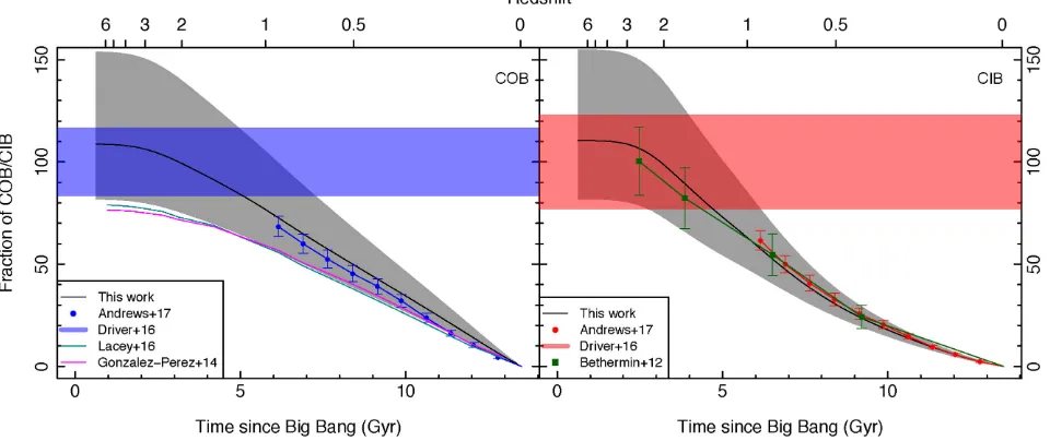
Figure 11. Contributions to the COB (left) and CIB (right) as a function of the age of the Universe relative to the total COB and CIB measured by Driver et al. (2016c), compared to measurements from Andrews et al. (2017b) and B´ethermin et al. (2012a) and predictions of the COB from Gonzalez-Perez et al. (2014) and Lacey et al. (2016). Bands indicate the respective uncertainty ranges.
wavelength. In the future, increasing amounts of TeV data will lead to stronger constraints on the shape of the COB – see Biteau & Williams (2015) for an early compilation of measurements. Ad-ditionally, observations of PeV gamma-rays will lead to similar constraints on the CIB via the same method.
6.3 The cosmic optical and infrared backgrounds
We can now break down the EBL into its two key components – the COB and CIB, respectively – by integrating under the respec-tive model curves over the relevant wavelength ranges. Given that
GALFORM does not model the mid-infrared, we limit ourselves to
comparing the semi-analytic model predictions with the observa-tions in the ultraviolet to the near-infrared only.
Our model (see Fig.11) predicts a roughly equal split between the COB and CIB, in line with observations (see Driver et al.2016c
and compilation within). We predict integrated values for the COB and CIB of 26.0+−106.5.7and 28.0+
11.2
−7.2 nW m−2sr−1respectively for the current epoch, and a peak value for the COB of 12.6+−53..64nW m−2sr−1at 1.19µm at the current epoch. This is in agreement with H.E.S.S. and MAGIC, which find maximum values of 15.0±3.6 and 12.75+−22..2975 nW m−2 sr−1, respectively, both at 1.4µm. The Gonzalez-Perez et al. (2014) iteration ofGALFORMunderpredicts the integrated COB by about 35 per cent, yielding an integrated value of 15.8 nW m−2sr−1, while the Lacey et al. (2016) model predicts 16.7 nW m−2sr−1. Both models also reach peak values of the COB below the H.E.S.S. and MAGIC observations – 7.7 nW m−2sr−1 atλ=1.18µm and 8.0 nW m−2sr−1at 1
.36µm for the Gonzalez-Perez and Lacey models, respectively. For comparison, the Gilmore et al. (2012) model obtains 29.0 and 27.0 nW m−2 sr−1 for the integrated COB and CIB, respectively, and predicts a peak value of the COB of 12.7 nW m−2sr−1at 1.28µm. Our model predicts an AGN contribution of approximately 0.6 nW m−2sr−1or 2.5 per cent (approximately equally split between obscured and unobscured AGN) to the integrated COB and 1.4 nW m−2sr−1or 5.1 per cent to the integrated CIB (mostly from obscured AGN).
Finally, our model predicts a CIB of 0.53−+00..2415nW m−2sr−1at 850µm, in line with the 0.43−+00..2415 nW m−2sr−1 observed using galaxy number counts from SCUBA-II (Chen et al. 2013b) and 0.50−+00..2319nW m−2sr−1from direct observations using theCosmic
Background Explorer(Fixsen et al.1998). The Gonzalez-Perez et al. (2014) and Lacey et al. (2016) models also show good agreement, predicting 0.44 and 0.54 nW m−2sr−1, respectively. The CIB at this wavelength primarily originates from galaxies atz=1−3 (Zavala et al.2017), lending confidence to the predictions of all models at higher redshifts.
Fig.11shows the accumulation of the COB and the CIB as one looks back in time. All model contributions to the CIB agree very well with both the Andrews et al. (2017b) and B´ethermin et al. (2012a) measurements, while the phenomological model slightly overpredicts the COB relative to Andrews et al. (2017b). The phe-nomological model reaches final values of the COB and CIB fully consistent with Driver et al. (2016c). The figure also shows the un-derprediction of the COB byGALFORM. This is not surprising given the deficit of theGALFORM predicted CSED below the phenomo-logical model (see Figs5and6), supporting the predictions of the phenomological model.
Figure 12. The comoving IGL, COB and CIB as a function of cosmic time for the phenomological model and Gilmore et al. (2012) with predictions for the COB from Gonzalez-Perez et al. (2014) and Lacey et al. (2016). The Driver et al. (2016c) measurements atz=0 are shown for comparison. Bands indicate the respective model uncertainty ranges.
6.4 Stellar mass growth
While the phenomological model is focused and calibrated to en-ergy, it is also capable of providing a complete description of stellar and dust mass evolution.
Fig.13shows the predicted buildup of stellar mass as a function of time for spheroids and discs (more precisely, the material that exists in spheroids and discs today). We show two curves – total stellar mass formed, computed by integrating the CSFH fitting func-tions (dashed lines, with bands to indicate the model uncertainty) and mass surviving at the specified time (solid lines). The curves differ as stellar material is returned to the ISM by supernovae and winds of thermally pulsating asymptotic giant branch stars. The Bruzual & Charlot (2003) models return from 35 per cent at 1 Gyr to 44 per cent at 10 Gyr of stellar mass to the ISM and place 8 per cent at 1 Gyr to 14 per cent at 10 Gyr into stellar remnants.
The green and blue points represent the total stellar mass density as reported by Moffett et al. (2016a) and Wright et al. (2017). The Moffett et al. (2016a) integrated stellar mass estimates have a 32 per cent uncertainty, equally portioned (22 per cent each) between un-certainty in the fitted functions and cosmic sample variance. The model predicts an almost equal distribution of stellar mass residing in discs (49.9 per cent) and spheroids (50.1 per cent), reproduc-ing the 47–53 per cent stellar mass ratio of Moffett et al. (2016b). (‘Little blue spheroids’ are deemed to be disc material.) We do not have to adjust the spheroid star formation history by 25 per cent akin to Driver et al. (2013). Note that the spheroid to disc mass ratio is independent of cosmic variance, barring large hidden clustering effects. We also note that the total stellar mass in spheroids enters a slow decline sincet=5 Gyr with the total stellar mass levelling off att∼10 Gyr, in agreement with Driver et al. (2013).
[image:16.595.50.284.61.285.2]We supplement Fig.13 with predictions derived by Guo et al. (2016) from the Gonzalez-Perez et al. (2014) version of GAL-FORMand theEAGLE suite of hydrodynamic simulations (Schaye et al.2015). Briefly, theEAGLEsimulation used by Guo et al. (2016)
Figure 13. Stellar mass as a function of cosmic time in the empirical model, with mass formed (dashed lines) and mass surviving (solid lines, with bands to indicate the model uncertainty) for spheroids (red), discs (blue) and both combined (black). The total mass in stellar remnants for both components is shown in cyan. The green, blue and orange points represent the Moffett et al. (2016a), Wright et al. (2017) and Driver et al. (2017) stellar mass measurements, respectively, while the faint red and grey points represent the Madau & Dickinson (2014) and Wilkins, Trentham & Hopkins (2008) compilations. Also shown are predictions fromGALFORM(dark green) and EAGLE(purple).
consists of a (100 cMpc)3box populated by 15043particles of both gas and dark matter.EAGLE uses a Chabrier (2003) IMF and the Bruzual & Charlot (2003) stellar libraries to derive mock photom-etry and stellar masses. The phenomological model predicts stellar mass equally as good asGALFORM, and matches the low-redshift data better thanEAGLE.
6.5 Dust mass growth
Using the phenomological model, we can also arrive at predictions of the dust mass density from the normalization constant used to scale up the Dale et al. (2014) templates to the total energy absorbed and re-released into the far-infrared. Two parameters are necessary to do so – the mass of a gas particle with respect to the mass of a hydrogen atommgas/mHand the dust to gas mass ratioMdust/Mgas. We assumemgas/mH=1.3 andMdust/Mgasthat scales linearly with the generating function for the metallicity of newly formed stars (i.e. the total stellar mass formed, see Fig.2) to reachMdust/Mgas=10−2.5 atz=0. The assumedMdust/Mgasratio atz=0 value is within the range ofMdust/Mgas observed in nearby galaxies by theHerschel Reference Survey (Cortese et al.2016), whilemgas/mH= 1.3 is assumed by the same to account for helium in the ISM.