Reliability Evaluation of the Minimum Spanning Tree on Uncertain Graph

Reliability Evaluation of the Minimum Spanning Tree on

Uncertain Graph

Jie Tang

1

_{, Yuansheng Liu}

1*

_{, Zhonghua Wen}

2

1 _{Ministry of Education Key Laboratory of Intelligent Computing and Information Processing, College of}

Information Engineering, Xiangtan University, Xiangtan 411105, Hunan, China.

2_{Department of Computer & Communication, Hunan Institute of Engineering, Xiangtan 411104, Hunan,}

China.

* Corresponding author. Tel.: 13636550479; email: [email protected] Manuscript submitted June 6, 2014; accepted October 29, 2014.

doi: 10.17706/jcp.10.1.45-56

Abstract: Minimum spanning tree is a minimum-cost spanning tree connecting the whole network, but it couldn't be directly obtained on uncertain graph. In this paper, we define the reliability as the existence probability of all minimum spanning trees and present an algorithm for evaluating reliability of the minimum spanning tree on uncertain graph. The time complexity of the algorithm is O(Nmn), where n, m and N stand for the number of vertices, edges and minimum spanning trees, respectively. Because this algorithm spends more time finding minimum spanning tree, we propose an improved algorithm whose time complexity is O(Nm). The improved algorithm uses disjoint set data structure so that the average time complexity on finding a new minimum spanning tree is O(m/n). The two algorithms are analyzed in detail and the experiment results agree with theoretical analysis.

Key words: Implicated graph, minimum spanning tree, uncertain graph.

1.

Introduction

IN graph theory, a spanning tree of an undirected graph is a tree that contains all the vertices. A minimum spanning tree (MST) of an edge-weighted graph is a spanning tree with the minimum sum of edge weights among all spanning trees. Many practical problem can be modeled by using MST, and it has been widely applied in many fields such as wireless sensor networks [1], [2], cluster analysis [3]-[5] and data storage [6].

There have been many studies of the MST problem dealing with deterministic graphs and have been designed some well known algorithm such as Kruskal [7] and Prim [8], in which the MST problem can be solved in polynomial time. In deterministic graph, all edges are assumed to be fixed, but such an assumption might not always be right. For example, the links in wireless sensor network (WSN) may be impassable caused by noise, collision and congestion, we can use uncertain graph to represent the WSN.

Some researchers assume that each edge of an uncertain graph has an existence probability. An uncertain graph is also refereed to as a probabilistic graph [9]. Each possible subgraph of the uncertain graph is called implicated graph. Their research mainly focus on graph mining [10]-[12], graph queries [13]-[15] and basic graph structure [16], [17].

MST (PMST) problem, fuzzy MST (FMST) problem and interval data MST (IDMST) problem. Many efficient algorithms have also been developed by some researchers [18]-[20].

In multicast routing protocols, MST is one of the most effective methods to multicast the massages from a source node to the destinations. When a connected link goes down, the network topology need to be updated. So evaluating the reliability of MST is significant. In this paper, we assume that each edge of a uncertain graph has a existence probability and a weight. The existence probabilities might represent the fault possibility in links and the edge weights represent time or cost. We try to evaluate the reliability of MST, which is the existence probability of all MSTs.

The number of implicated graph increases exponentially with the number of edges, it need take a lot of time if we enumerate each implicated graph. In this paper, we propose a fundamental algorithm, called FERM (Fundamental algorithm of Evaluating the Reliability of MST), and an improved algorithm (IERM) to evaluating the reliability of the MST. The two algorithms classify all implicated graphs by finding all MSTs. The improved algorithm uses disjoint structure and search algorithm to get the swap-edges of each edge, so that the time complexity required to find a new MST is O(m/n). Thus, the improved algorithm is more than n times as fast as the fundamental algorithm in theory.

The remaining of this paper is organized as follows. Section 2 gives the problem formulation. In Section 3, two algorithms for reliability evaluation of MST on uncertain graph are presented. We report our experiment result in Section 4, and a conclusion reached in Section 5.

2.

Problem Formulation

Definition 1 (Uncertain graph): An uncertain graph ( , ,V E W P, ), is defined over a set of vertices V, a set of edges E, a set of edge weights W { ( )|w e eE w e, ( ) }, and a set of probabilities

{ ( )| , ( ) (0,1]}

P p e eE p e  of edge existence.

An implicated graph

G



(

V

G

,

E W

G

,

G

)

of an uncertain graph is an certain graph which is realized

by sampling each edge in according to the probability

p e

( )

. We denote the relationship between

G

and as



G

. Clearly, we have

V

G



V

,

E

G



E

and WG { ( )|w e eEG}W . There are a total

of | |

2

E implicated graphs, because each edge provides us with a binary sampling decision. Following the

same assumption of the existing uncertain graph models [10], [13], [21], we assume that uncertain variables of different edges are mutually independent. Based on this assumption, the probability of sampling the implicated graph G from the uncertain graph is

Pr( ) ( ) (1 ( )).

G G

e E e E E

G p e p e

 

 







Let Imp( ) denotes the set of all implicated graphs of the uncertain graph . Moreover, it is easy to

know that function Pr( G) defines a probability distribution over Imp( ).

Fig. 1(a) shows an uncertain graph 1. The two numbers on each edge represent weight and existence

probability, respectively. The uncertain graph ₁ has 5

2

implicated graphs because ₁ has five edges.

Fig. 1(b) shows an implicated graph of the uncertain graph 1, which shows in Fig. 1(a), and the sampling

probability of the implicated graph is p e( )2 p e( )3 p e( )4 p e( ) (15  p e( )))1 0.03528.

Definition 2 (Main implicated graph): Given an uncertain graph ( , ,V E W P, ), we define the

Fig. 1(c) shows the main implicated graph of ₁. It is clear that the main implicated graph has three MSTs {e1e2e3}, {e2e3e4} and {e2e4e5} and the total weight of any MST is equal to 4.

Definition 3 (Reliable implicated graph): Given an uncertain graph ( , ,V E W P, ). Let G be any implicated graph of , T be an MST of implicated graph G and G _{( )}

e T

W w e







be the weight of the MST T. If

ˆ

G G

W W , then

G

is a reliable implicated graph of the uncertain graph .

A B C D 2,0. 9 _1,0 .7

2,0.8

1,0_.9 e1 e2 e4 e3 2,0.7 e5 A B C D e2 e4 e3 e5 A B C D 2 1 2 1 e1 e2 e4 e3 2 e5

(1) (2) (3)

Fig. 1. Example: (a) uncertain graph ; (b) an implicated graph of 1; (c) Main implicated graph of 1.

Definition 4 (Reliability of MST): Given an uncertain graph ( , ,V E W P, ) . Let

ˆ

{ | ( ) G G}

R G GImp W W denotes the set of all reliable implicated graph of the uncertain graph .

The reliability of MST on uncertain graph can be defined as follows:

Pr( ).

G R

r G









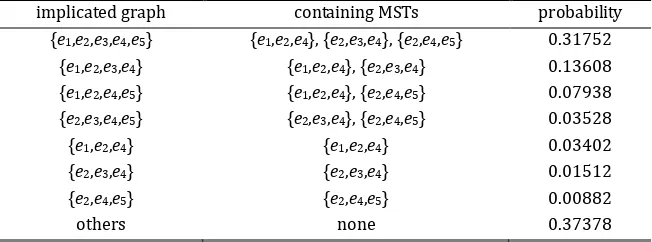
Table 1. Reliability Evaluation of the MST on Uncertain Graph Fig. 1(a).

implicated graph containing MSTs probability

{e1,e2,e3,e4,e5} {e1,e2,e4}, {e2,e3,e4}, {e2,e4,e5} 0.31752

{e1,e2,e3,e4} {e1,e2,e4}, {e2,e3,e4} 0.13608

{e1,e2,e4,e5} {e1,e2,e4}, {e2,e4,e5} 0.07938

{e2,e3,e4,e5} {e2,e3,e4}, {e2,e4,e5} 0.03528

{e1,e2,e4} {e1,e2,e4} 0.03402

{e2,e3,e4} {e2,e3,e4} 0.01512

{e2,e4,e5} {e2,e4,e5} 0.00882

others none 0.37378

Table 1 shows the existence probability of the implicated graph, which contains at least one MST in {e2e4e5}, {e1e2e4} or {e2e4e5}. There are seven implicated graphs containing MST, so the reliability of the MST is 0.62622.

3.

The MST Reliability Evaluation

3.1.

Fundamental Algorithm

Theorem 1: Given an uncertain graph ( , ,V E W P, ). Let n be the number of vertices of uncertain graph , respectively,

T



{ ,

e e

_{1 2}

,

,

e

_n1

}

be an MST of the main implicated graph Gˆ and

1 2

{ ,

,

, }

i i

A



e e

e

, where i{1, ,n1}. We define

1

1

{ | ( ) }, 0,

{ | ( ) }, 0 1,

{ | ( ) }, 1,

G

i i G i G

i G

G G Imp e E i

D G G Imp A E e E i n

G G Imp A E i n

That is,

D

i represents a set of graph whose edge set contains set

A

i and excludes edge

e

i1(if exists)

and these graphs in set

D

i are a subgraph of the main implicated graph

G

ˆ

. Then, we have the following

two results: 1) 1

0 ( ) n i i D Imp   

2) D_iD_j , where i j

Proof: We prove the two parts separately:

1) For any implicated graph G_iImp( ) , if

1

{

,

,

,

}

i j j y

G x x x

E

T

e

e

e



 

, where

1( 1, 2,..., 1) j j

x x j y , then there must exist a k meet:

1 1

1,

,

1,

1.

j j j j

x

x

j

k

x

x

j

k

 









 



 



Then, we have the following:

0 1 1

,

1,

,

1.

i i k

G

D

x

G

D

x







 





So we have 1 0 ( ) n i i Imp D  

 . According to Equation (1), we have 1 0 ( ) n i i D Imp    .

2) According to Equation (1), we have D_iD_j{ |G GImp( )A_jE_Ge_i1E_G}. However, A_jE_G

and

e

_i1



E

_G can't be achieved at the same time since

e

_i1



A

_j. Thus,

i j

DD  .

Corollary 1: Let

I



{ ,

e e

_{1 2}

,

, }

e

_k and

O



E

. Now assume that there exist a minimum spanning

tree

T



{ ,

e e

1 2

,

,

e

n1

}

s.t.

I



T

and T  O . Let S{ |G GImp( ) I EG O EG  }, we

define

{ | }

i i G i G

D  G G  S I E O E  

where

I

i

 

I

{

e

k1

,

e

k2

,

, }

e

i , Oi O {ei1}. Then, we have

1 n i i k D S    .

According to Corollary 1,

Imp

( )

can be divided recursively until each implicated graph in set

S

contains the same MST, namely,

I



T

. It is clear that the existence probability of set

S

is

( ) (1 ( ))

 

 





e I e O

p e p e . We'll call the function GetMST to get a minimum spanning tree whose edge set

contains set I and exclude set O, which is implemented by Kruskal' or Prim's algorithm. The fundamental algorithm, called FERM (Fundamental algorithm of Evaluating the Reliability of MST), is outlined as following:

Example 1: Fig. 2(a) is an uncertain graph 2 and Fig. 2(b) is a minimum spanning tree of its main

implicated graph. It is obvious that when all edge weights have different values, the MST must be unique, so the edge weights in Fig. 2(a) are set as 1 or 2 to better understand function call RMST( , , ₂). Fig. 3

builds a multiway-tree to simulate function call

RMST

( ,

 

,

2

)

. The nodes with bold bolder show that

the algorithm has already found a set of reliable implicated graph. As we can see from Fig. 3, all reliable implicated graphs are divided into nine nodes. However, the uncertain graph 2 has

6

2



64

implicated

Algorithm 1 The FERA algorithm

Comment Calls from RMST( , , ) 

1. Procedure RMST I O( , , ) > ( , ,V E W P, )

2. TGetMST I O( , , )

3.

k



the number of elements of set I

4.

r



0

5. IF Gˆ

e T W



THEN

6. IF

T



I

THEN

7. _{( ) (1 ( ))}

e I e O

r



 p e



 p e

8. ELSE

9. FOR

i



k

TO

|

V

| 1



DO

10. I_i I {e_k1,e_k2, , }e_i

11. O_i O {e_i₁}

12. r r RMST I O( ,_{i i}, )

13. RETURN r

1

2 3

4

1,0.7

2

,0

.7

1,0.

6 1,0

.8

2,0_.9

e1

e2

e3

e4

e5

2,0.9 e6

1

2 3

4

e1

e2

e4

(a) (b)

Fig. 2. Example: (a) uncertain graph ₂; (b) an MST of main implicated graph of Fig. 2(a).

e1 e2 e1e2 e4 e1e2e4

e1

e1e2 e2 e1e3 e2e3 e1e4 e2e3e4 e1 e1 e2e3 e1e3 e2e4 e1e3e4 e2 e1e2 e4e5 e1e2e5 e4

e2e3 e1e4e5 e2e3e5 e1e4 e1e3 e2e4e5 e1e3e5 e2e4

e2e3 e1e4e5e6 e2e3e6 e1e4e5 e1e3 e2e4e5e6 e1e3e6 e2e4e5

e1e2 e4e5e6 e1e2e6 e4e5

0.1568

0.06048

0.006048

0.1008

0.03888

0.003888

0.294

0.1134

0.01134

I O

Fig. 3. The recursive procedure of the function call RMST( , , 2).

Theorem 2: The time complexity of the Algorithm 1 is O(Nnm), where N denotes the number of MSTs included in main implicated graph

G

ˆ

, n and m denote the number of vertices and edges, respectively.

Proof: Note that each time the function RMST is called, it will call the function GetMST once and

produces at most n-1 recursive calls. So the total number of function call RMST is at most

Nn

 

1

Nn

.

However, it requires O(m) time to solve an MST problem. Thus, the total time complexity is O(Nnm).

3.2.

Improved Algorithm

designs an improved algorithm, called

IERM

(Improved algorithm of Evaluating the Reliability of MST), to obtain a new MST by performing edge replacement operation on previous MST. Let ₁ e ₂

T





T

denotes

the edge replacement operation, where

T

2 is the result of

T

1 after the edge replacement operation,

2 1

{ }

{ }

T

 

T

e



e

, and

e



is the swap-edge of

e

.

Theorem 3: Assume that

T

_a is a spanning tree and

T

_b is an MST of implicated graph G. Let

1 2

{ ,

,

, }

_k

I



e e

e

denotes the set of different edges, where

e

i



T

a and

e

i



T

b. We can perform the

edge replacement operation k times, and then obtain

1 2

0 1 2 1

( )

e e

,

,

ek

( ),

a k b k

T T



 

T

T

T

_



T T

and

1

( )

( ).

i i

e T e T

w e

w e



 







Proof: For

i



1 ~

k

, repeat the following two steps:

1) Delete

e

_i from

T

_i1, and then the tree

T

_i1 divided into two connected-components

V

₁ and

V

₂.

2) Assume that the path from vertex u to v in tree

T

b is

u u

(

0

)



u

1

,

,

u

x1

,



v u

(

x

)

, denotes as

u v

P

. There must exist

i i

(



x

)

such that

u

i



V

1 and

u

i1



V

2. Let

e

 

i

( ,

u u

i i1

)

. Because of

T

b

is a MST, it is easy to know that

w e

( )

i

 

w e

( )

i , 1 i

e

i i

T

_





T

, and

1 1

( ) ( ) ( ) ( ) ( )

i i i

i i

e T e T e T

w e w e w e w e w e

 

  



   







.

Thus, this theorem is proven.

Theorem 4: Let T be an MST included in graph G. Assume that edge

e T



connects two connected-components, called

V

1 and

V

2, then for any MST

T



whose edge set doesn't contain edge e,

there exists an edge

e





( , )

u v

 

such that

u



V

1,

v



V

2 and

w e

( )

 

w e

( )

.

Let

e



( , )

u v

. Assume that the path

P

_vu in tree

T



is

u u

(

0

)



u

1

,

,

u

x1

,



v u

(

x

)

. Then, there

must exist

i i

(



x

)

such that

u

i



V

1 and

u

i1



V

2. Assume

e

 

( ,

u u

i i1

)

, we have  If

w e

( )

 

w e

( )

, let *

{ } { }

T  T e e , then we has *

( ) ( )

e T e T

w e w e

  







.

 If

w e

( )

 

w e

( )

, let *

{ } { }

T  T e e , then we has *

( ) ( )

e T e T

w e w e

 







.

The above two situations obviously contradict the fact that T and

T



are an MST. Therefore, we have

( )

i

( )

w e



w e

.

Assume that E V V G( ,_{1 2}, ) {e E e V_G|  ₁ V₂}. According theorem theorem 4, if there exists

e



, such that eE V V G( ,_{1 2}, ) and w e( ) w e( ), then we can obtain a new MST by edge replacement operation, that is

newT

 

T

{ }

e



{ }

e

. Otherwise, the graph G doesn't exist any other MST whose edge set doesn't

contain the edge e.

To find swap-edges of each edge in tree T, we could traverse all edges in graph G from small to large according to its weight. For each edge *

e



G

, we will perform the following two steps: 1) Let * * *

(

,

)

e



u v

, then traverse the path ** u v

edges whose weights are equal to *

( )

w e

.

2) Use disjoint structure to compress the path ** u v

P

.

To find the path between two vertices of tree T, we should know the relationship (parent-child, brotherhood or other) of two vertices firstly. Assume that vertex 1 is root-node, the function

GetChild

is defined as follow:

( , ) { | is a child-node of in }

GetChild T w



v v

w

T

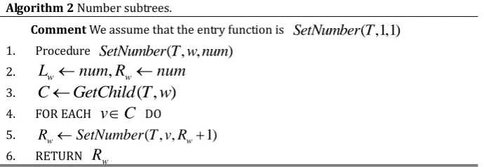
The following algorithm numbers each subtree of the tree T:

Algorithm 2 Number subtrees.

Comment We assume that the entry function is SetNumber T( ,1,1)

1. Procedure SetNumber T w num( , , )

2.

L

w



num R

,

w



num

3.

C



GetChild T w

( , )

4. FOR EACH

v



C

DO

5. R_w SetNumber T v R( , , _w1)

6. RETURN

R

_w

Definition 5 (Least common ancestor): Let T be a rooted tree. The least common ancestor between two vertices v and w is defined as the lowest node in T that has both v and w as descendant-nodes (where we allow a vertex to be a descendant-node of itself)

Example 2: Fig. 4 shows an MST T and execution result from function call

SetNumber T

( ,1,1)

.

According the Algorithm 2, we know that

L

i is generated by pre-order traversal and

max{ |

i j

R



L

vertex

j

is descendant-node of vertex

i

}

.

L1: 1

L2: 2

L3: 5

L4: 3

L5: 4

L6: 6

L7: 7

R1: 7

R2: 4

R3: 7

R4: 3

R5: 4

R6: 6

R7: 7

1

2 3

4 5 6 7

4

3

2 4 5 8

Fig. 4. An MST T & Number ranges of each subtree.

Example 2 shows that if

L

_j



[ ,

L R

_{i i}

]

, then vertex j is descendant-node of vertex i. Assume that

1

,

2

u u



T

, we take the following steps to find the path between vertex

u

1 and

u

2:

1) Traverse these vertices from

u

1 to

1

until we find a vertex v such that

L

u₂



[

L R

v

,

v

]

.

2) Traverse these vertices from vertex

u

2 to

v

.

Therefore, 1 2 u u

P

can be represented as

u

1



 

v



u

2. It's clear that vertex v is the least

common ancestor(LCA) between two vertices

u

1 and

u

2.

Next, we use disjoint structure to compress the path 1 2 u u

P

. Let

RT

i be current LCA of vertex i, then for

any vertex w in the path 1 2 u u

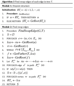
father-node of vertex x in tree T. Thus, the algorithm of finding swap-edges shows as Algorithm 3.

Algorithm 3 Find swap-edges of each edge in tree T.

Module 1: Disjoint structure

Initialization RT_ii i( 1, 2, , )n

1. Procedure GetRoot u( )

2. IF

u



RT

_u THEN RETURN

u

3. ELSE RETURN

(

RT

_u



GetRoot RT

(

_u

))

Module 2: Find swap edges

1. Procedure

FindSwapEdge G T

( , )

2.

S

 

3. FOR EACH

e



( , )

u v



E

_G DO

4.

lca



ru



GetRoot u

( )

5.

rv



GetRoot v

( )

6. WHILE

rv



[

L

_lca

,

R

_lca

]

DO

7.

f



GetFather T lca

( ,

)

8.

lca



GetRoot f

( )

9. Let

P

_rvru be

ru

 

lca

 

rv

10. FOR EACH edge

e



in path ru

rv

P

DO

11. IF

w e

( )

 

w e

( )

THEN

12.

S

 

S

{( , )}

e e



13. FOR EACH vertex

w

in path

P

_rvru DO

14.

RT

_w



lca

15. RETURN

S

Example 3: Assume that e₁(2, 5),e₂(3, 6),e₃(4, 5),e₄(5, 6), ( )w e₃ 4, ( )w e₄ 5 and

e e

3

,

4



G

, as

shown in Fig. 5. We first find the path between vertex 4 and 5 because of w e( )₃ w e( )₄ , it's clear that the

edge

e

3 is a swap-edge of edge

e

1 as

w e

( )

1



w e

( )

3 , then we replace the two vertices 4 and 5 with their

LCA, that is RT₄2 and RT52. Next, we deal with the edge

e

4, we can assume that e4(5, 6)(2, 6)

because of RT52. So it is easy to know that S{( , ), ( ,e e1 3 e e2 4)}.

1

2 3

4 5 ₆ 7

4

3

2 4 5 8

1

2

3

6 7

4

3

5 8

1

7

8

4

5

Fig. 5. The path-compressed procedure.

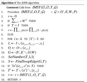
From what mentioned above, the improved algorithm is outlined as Algorithm 4.

Theorem 5: The time complexity of the improved algorithm is O(Nm).

spanning tree is O(m/n), so the time complexity of the improved algorithm is O(Nn*(m/n)=O(Nm).

Algorithm 4 The IERM algorithm

Comment Calls from

IMST

( , , , )

 

T

1. Procedure

IMST I O T

( , , , )

>



( , ,

V E W P

, )

2.

r



0

3. IF Gˆ

e T W



THEN

4. IF

T



I

THEN

5. r



_{e I} p e( )



_{e O} (1p e( ))

6. ELSE

7. FOR

i



k

TO

|

V

| 1



DO

8.

I

i

 

I

{

e

k₁

,

e

k₂

,

, }

e

i

9.

O

_i

 

O

{

e

_i1

}

10.

G



( ,

V E

O W

,

)

11.

SetNumber T

( ,1,1)

12.

S



FindSwapEdge G T

( , )

13. IF



e



((

e

_i1

, )

e





S

)

THEN

14.

T



 

T

{ }

e



{

e

i₁

}

15.

r

 

r

IMST I O T

( ,

_{i i}

,



, )

16. RETURN

r

4.

Experiment Results

For the experiments, we utilize the block-random graph mode [22], which can generate both the Erdos-Renyi random graph and Scale-free random graph. The existence probabilities of each edge are uniformly generated between 0 and 1. These algorithms were implemented in C++, all experiments were performed on an HASEE K470P-i5 notebook with 2.4GHz CPU and 4GB RAM, running Windows 7.

Experiment 1: We consider that the main implicated graph is a complete graph with edge weights fixed at the same value. In this case, all the spanning trees are MSTs, and the total number of spanning tree is

2 n

n

 according to theorem by Cayley [23].

Table 2 shows the results of two algorithms, N denotes the number of MSTs in the main implicated graph,

n

K

denotes that the main implicated graph is a complete graph with n vertices; the values Ratios denote the ratio of FERM to IERM. According to the theoretical analysis, the time complexity of algorithm FERM should be n times faster than algorithm IERM, but the code implementation to algorithm IERM is more complex, so the actual ratios Ratios are lower than the expected ratios.

Table 2. The Performance Evaluation in the Same Weight for

K

_n

Time(s)

G N FERM IERM Ratios Reliability

K5 125 0.00100 0.00100 1.0 0.729287

K6 1296 0.00500 0.00500 1.0 0.949277

K7 16807 0.08100 0.07000 1.1 0.812293

K8 262144 1.35800 1.06700 1.2 0.981199

K9 4782969 29.2060 22.1580 1.3 0.990147

K10 100000000 671.767 521.091 1.3 0.990147

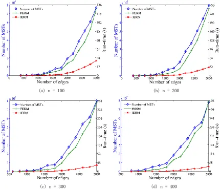
distances are not all the same in the real world. In order to analyze the effect of the number of vertices and edges on the run-time, the experiment changes the number of vertices and edges, respectively. Fig. 6 shows run-time comparison chart for algorithms FERM and IERM. In the four subgraphs, the number of vertices is set to 100, 200, 300 and 400, respectively.

As the figure shows, the time cost of algorithm IERM is unrelated to the number of vertices, the run-time ratios of FERM to IERM increases with the number of vertices and edges. In Fig. 6(a), when the number of edges is equal to 3000, the value N*m of the algorithm IERM is approximately equal to 2.1 million and the run-time is approximately equal to 28 seconds. Due to the complexity of the code, the run-time of the algorithm IERM agree with the experiment data. when the number of vertices is 400 and the number of edges is 3000, algorithm IERM is 14 times faster than algorithm FERM.

(a) n = 100 (b) n = 200

(c) n = 300 (d) n = 400

Fig. 6. The performance evaluation with different number of vertices.

5.

Conclusions

This paper investigates the problem of evaluating reliability of the minimum spanning tree on uncertain graph for the first time and designs two algorithms to solve this problem base on classifying implicated graphs. The improved algorithm IERM proposes a novel approach to obtain a new MST, which time complexity is O(m/n). The experiment results verify the efficiency of this algorithm and accuracy of theoretical analysis.

This work was supported in part by the National Natural Science Foundation of China (GrantNo.61272295, GrantNo.61105039, and GrantNo.61202398), Hunan Provincial Innovation Foundation For Post-graduate (No. CX2014B276).

References

[1] Khan, M., Pandurangan, G., & Kumar, V. A. (2009). Distributed algorithms for constructing approximate minimum spanning trees in wireless sensor networks. IEEE Transactions on Parallel and Distributed Systems, 20(1), 124-139.

[2] Saravanan, M., Ravi, R., & Prabaharan, S. (2013). A survey on distributed algorithms for constructing minimum spanning trees in wireless sensor networks. American-Eurasian Journal of Scientific Research, 8(4), 192-197.

[3] Zhong, C., Miao, D., & Wang, R. (2010). A graph-theoretical clustering method based on two rounds of minimum spanning trees. Pattern Recognition, 43(3), 752-766.

[4] Barzily, Z., Volkovich, Z., Akteke-Öztürk, B., & Weber, G. W. (2009). On a minimal spanning tree approach in the cluster validation problem. Informatica, 20(2), 187-202.

[5] Päivinen, N. (2005). Clustering with a minimum spanning tree of scale-free-like structure. Pattern Recognition Letters, 26(7), 921-930.

[6] Li, J., Yang, S., Wang, X., Xue, X., & Li, B. (2009, July). Tree-structured data regeneration with network coding in distributed storage systems. Proceedings of IWQoS. 17th International Workshop on Quality of Service (pp. 1-9).

[7] Kruskal, J. B. (1956). On the shortest spanning subtree of a graph and the traveling salesman problem. Proceedings of the American Mathematical Society: Vol. 7. No. 1 (pp. 48-50).

[8] Prim, R. C. (1957). Shortest connection networks and some generalizations. Bell System Technical Journal, 36(6), 1389-1401.

[9] Hintsanen, P., & Toivonen, H. (2008). Finding reliable subgraphs from large probabilistic graphs. Data Mining and Knowledge Discovery, 17(1), 3-23.

[10]Zou, Z., Li, J., Gao, H., & Zhang, S. (2010). Mining frequent subgraph patterns from uncertain graph data. IEEE Transactions on Knowledge and Data Engineering, 22(9), 1203-1218.

[11]Zou, Z., Gao, H., & Li, J. (2010, July). Discovering frequent subgraphs over uncertain graph databases under probabilistic semantics. Proceedings of the 16th ACM SIGKDD International Conference on Knowledge Discovery and Data Mining (pp. 633-642).

[12]Papapetrou, O., Ioannou, E., & Skoutas, D. (2011, March). Efficient discovery of frequent subgraph patterns in uncertain graph databases. Proceedings of the 14th International Conference on Extending Database Technology (pp. 355-366).

[13]Potamias, M., Bonchi, F., Gionis, A., & Kollios, G. (2010). K-nearest neighbors in uncertain graphs. Proceedings of the VLDB Endowment: Vol. 3, No. 1-2 (pp. 997-1008).

[14]Dimitrov, D., Singh, L., & Mann, J. (2013, January). Comparison queries for uncertain graphs. Database and Expert Systems Applications, 124-140.

[15]Ruan, W., Wang, C., Han, L., Peng, Z., & Bai, Y. (2013). Uncertain subgraph query processing over uncertain graphs. Web Technologies and Applications, 132-139.

[16]Zou, Z., Li, J., Gao, H., & Zhang, S. (2010, March). Finding top-k maximal cliques in an uncertain graph. Proceedings of IEEE 26th International Conference on Data Engineering (ICDE) (pp. 649-652).

[19]Janiak, A., & Kasperski, A. (2008). The minimum spanning tree problem with fuzzy costs. Fuzzy Optimization and Decision Making, 7(2), 105-118.

[20]Chen, X., Hu, J., & Hu, X. (2009). A polynomial solvable minimum risk spanning tree problem with interval data. European Journal of Operational Research, 198(1), 43-46.

[21]Zou, Z., Li, J., Gao, H., & Zhang, S. (2009, November). Frequent subgraph pattern mining on uncertain graph data. Proceedings of the 18th ACM Conference on Information and Knowledge Management (pp. 583-592).

[22]Karrer, B., & Newman, M. E. (2011). Stochastic blockmodels and community structure in networks. Physical Review E, 83(1), 016107.

[23]Cayley, A. (1889). A theorem on trees. Quart. J. Math, 23(376-378), 69.

Jie Tang received his B.S. degree in computer science and technology from Xiangtan University, Hunan, China in June 2012. He is currently working towards his M.S. degree in computer science at Xiangtan University, China. His current research interests includes uncertain graph and graph theory.

Yuansheng Liu received the B.S. degree in software engineering from Xiangtan University, Hunan, China, in 2012. He is currently working towards his M.S. degree in computer science and technology at Xiangtan University, China. His current research interests include date mining and machine learning.