ISSN: 2278-067X, Volume 1, Issue 3 (June 2012), PP.01-07
www.ijerd.com
1
Improvement the Performance Of Mobility Pattern In Mobile
Ad-Hoc Sensor Network using Qualnet 5.0
Manoj Rana
1, Shubham Kumar
2Upasana Sharma
3,
1
Assistant Professor and Head of Department,Computer Science Engineering Department, College of Engineering and Rural Technology Meerut, India
2
Assistant Professor, Computer Science Engineering Department, College of Engineering and Rural Technology Meerut, India
3
Assistant Professor, Computer Science Engineering Department, Amity University Noida, India.
Abstract––A mobile ad-hoc sensor network usually consists of large number of sensor nodes (stationary or mobile) deployed over an area to be monitored. Each sensor node is a self-contained, battery-powered device that is capable of sensing, communication and some level of computation and data processing. Due to the large amount usage of sensors in the network, it is important to keep each node small and inexpensive. This strictly restricts its resources in terms of energy, memory, processing speed bandwidth. We simulate the Mobile ad-hoc sensor network for its performance analysis. we introduced the concept of communication range remoteness for mobile nodes through random way point mobility model. We characterized the mobility of nodes with new mobility patterns through AODV protocol, without breaking the backward compatibility with earlier versions. In this paper we will proposed two model as non mobility model and mobility model. And in this paper we will compare both models using the concept of mobile ad-hoc sensor network. The performance through the multiple node of non mobility model was found better in comparison of mobility model. . than we design the concept of antenna and improve the frequency of transmitting signal for mobility model,this model is known as design mobility model. In this paper we improve the performance of design mobility in comparison of non mobility model and mobility model. The performance analysis of mobility and non-mobility and design mobility model is done through simulations on a commercial simulator called Qualnet version 5.0, software that provides scalable simulations of Wireless networks.
Keywords––AODV, CBR, LRPAN, WSN, FFD, RFD, Zig Bee.
I.
INTRODUCTION
A wireless sensor network usually consists of a large number of sensor nodes (stationary or mobile) deployed over an area to be monitored. Each sensor node is a self-contained, battery-powered device that is capable of sensing, communication and some level of computation and data processing. Due to the large amount usage of sensors in the network, it is important to keep each node small and inexpensive. This strictly restricts its resources in terms of energy, memory, processing speed and bandwidth. A wireless sensor network (WSN) is a wireless computer network consisting of spatially distributed autonomous devices using sensors to cooperatively monitor physical or environmental conditions, such as temperature, sound, vibration, pressure, motion or pollutants, at different locations. A sensor, in its simplest
definition, is a device that is capable of observing and recording a phenomenon. This is termed as sensing. Sensors are
used in various applications such as industry, military, healthcare, disaster relief, meteorology, etc. For example, sensors are used to study the formation of tornadoes by measuring the pressure, humidity, temperature, and wind direction when a tornado occurs. In rescue operations, seismic sensors are used to detect survivors caught in landslides and earthquakes. With advances in electronics, sensors now have the capability to sense, process, and communicate data. These small-sized sensor nodes have low cost, low power needs, and the ability to communicate over short distances. This has led to the development of sensor networks, which capitalize on the sensor node's ability to communicate. A sensor network consists of possibly several hundred sensor nodes, deployed in close proximity to the phenomenon that they are designed to observe. The position of sensor nodes within a sensor network need not be pre-determined. Sensor networks must have the robustness to work in extreme environmental conditions with scarce or zero interference from humans. This also means that they should be able to overcome frequent node failures. In this paper sensor node are mobiles deployed over the area so it is called mobile ad-hoc sensor network.
II.
OVERVIEW OF CURRENT LITERATURE
Some of the most important properties of a mobile user population are the characteristics and pattern of the user mobility. In simulating mobile systems, it is important to use a realistic mobility model so that the evaluation results from the simulation correctly indicate the real world performance of the system. A.K. Saha and D.B. Johnson [5] proposed a realistic model of node motion based on vehicular traffic, suitable for evaluating vehicular ad hoc networks. Y. Lu, H. Lin, Y. Gu, and A. Helmy [6] classified various mobility models, in addition to proposing the contraction, expansion, circling, hybrid contraction and random waypoint and hybrid Manhattan and RWP mobility models. These models covered scenarios in which nodes merge, scatter or switch to different mobility patterns over time. Mobility metrics like, node degree, link duration, relative speed, temporal dependence, and spatial dependence are studied to differentiate the characteristics of proposed and existing mobility models. They showed that average node degree and link duration are
T. Camp, J. Boleng, and V. Davies [7] investigated characteristics of different mobility models including
random walk, random waypoint, random direction, and reference point group mobility model. They compared these
mobility models using mobility metrics like data packet delivery ratio, average end to end delay, average hop count, control packet transmissions per data packet delivered and control byte transmissions per data packet delivered against average node speed. But the problem with this is that if the nodes are moving in the same direction with the same speed so we cannot have a better idea of the mobility of nodes as they seem static with respect to each other.
J. W. Wilson [8] combined several features of the existing individual and group mobility models to explore the sensitivity of routing protocol performance, to mobility patterns. Reference point group mobility model is combined with mobility vector model and the resulted model is used to examine sensitivity of existing ad hoc routing protocols, to changes in mobility generated by that model. Basic approach used is that, objects in real world react to accelerations. At each interval time in simulation, individual participant positions are calculated and their velocity vectors are adjusted. For different network participants maximum throughput is plotted against maximum velocity and a decrease in throughput is observed with increase in maximum participant velocity. This is due to the increased number of broken links due to increased average participant velocity. But for different mobility models we can have different link change rate and if nodes are moving with same velocity, we cannot have better idea of mobility.
There are two possible approaches to tackle the problem of designing realistic and reproducible mobility and communication models. In the first approach, mobility models are created that most closely represent the real world, after conceiving actual use of the systems. Although this approach guarantees realistic and relevant models but it could potentially lead to overly complex models that are hard to analyze. In the second approach, such models are created much like the creation of benchmark programs for computer systems. D.S. Tan, S. Zhou, J. Ho, J.S. Mehta, and H. Tanabe [9] used a combination of the two approaches and presented a general purpose method that may be used to reliably generate realistic mobility patterns with different characteristics. D. Shukla [10] investigated different mobility models and uses mobility parameters: average speed and distance traveled, transmission range and link changes, against average speed, to compare them
III.
ARCHITECTURE
The concept of wireless sensor networks is based on a simple equation: Sensing + CPU + Radio = Thousands of potential applications As soon as people understand the capabilities of a wireless sensor network, hundreds of applications spring to mind. It seems like a straightforward combination of modern technology. However, actually combining sensors, radios, and CPU’s into an effective wireless sensor network requires a detailed understanding of the both capabilities and limitations of each of the underlying hardware components, as well as a detailed understanding of modern networking technologies and distributed systems theory.
IV.
MOBILITY MODEL STRATEGIES
In WSNs, three different types of mobility have been suggested: random, predictable or fixed, and controlled.
Rand om Mobility
Random-walk mobility is assumed to be independent of the network topology, traffic flows and residual energy of nodes.
Predictable Mobility
The predictable or fixed trajectory of a mobile sink is fully deterministic as the sink always follows the same path through the network. In some cases, the path actually selected is, in fact, enforced by artificial or natural obstacles in the environment. One should observe that both in the case of random and predictable mobility, the actual speed of the sink can influence the amount of control data generated in the network, possibly limiting the benefits of sink mobility.
Controlled Mobility
In the case of controlled mobility, the path of the sink becomes a function of the current state of network flows and nodes’ energy consumption, and it keeps adjusting itself to ensure optimal network performance at all times. From the application perspective, controlled mobility can find its use in both continuous and event -base WSNs.
V.
SIMULATION ENVIRONMENT
Wireless Subnet: White cloud in the n/w is ZigBee subnet. This subnet is responsible for giving ZigBee properties to all the nodes.
Nodes: we consider a mobile ad-hoc sensor network with 10 mobile nodes and a statically placed data sink (root node). Data sink node (1) is a full function device and work as a PAN Coordinator.
Trffic Flow: We used the application of constant bit rate (CBR).We have taken node 2,3,4,5,6,7,8,910,11 as source and node 1 is taken in Scenario as sink node. We will send 300 packet of each size 50 bytes at start 1s. We have send all packet at 1s interval of time and ending time of simulation is 301s.
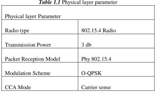
1 Physical layer parameters:The parameters used to configure PHY802.15.4 for FFD and RFD are
Table 1.1 Physical layer parameter
Physical layer Parameter
Radio type 802.15.4 Radio
Transmission Power 3 db
Packet Reception Model Phy 802.15.4
Modulation Scheme O-QPSK
CCA Mode Carrier sense
2 MAC Layer Parameters: The parameters used to configure MAC802.16e for FFD and RFD are:
Mac layer parameter
Mac protocol 802.15.4
Device type RFD(2-10)
Device type FFD(1)
FFD mode Pan Co-ordinator
Network layer parameters: At network layer IPv4 queue type is FIFO (First in First Out). AODV algorithm is used as routing protocol.
Application layer parameters: Constant bit rate application is run with packet size of 50 bytes and inter packet interval of 1s. Packet transmission starts at 1s and continue till end of simulation.
Scenario: In the model the components used are Wireless subnet, nodes configured and CBR traffic flow. Simulation parameters as shown below in table and all remaining parameters are by default.
VI.
SIMULATION RESULTS ANALYSIS
Running Scenarios for Non Mobility Model
Mobility Models: In this model sensor nodes are dynamic and pan co-coordinator are static In the performance evaluation of a protocol for a wireless sensor network, the protocol should be tested under realistic conditions including, but not limited to, a sensible transmission range, limited buffer space for the storage of messages, representative data traffic models, and realistic movements of the mobile users (i.e., a mobility model). This model is a journey through mobility models that are used in the simulations of mobile Ad-hoc sensor networks. Here the descriptions of mobility models that represent mobile nodes whose movements are independent of each other (i.e., entity Mobility models) and mobility models that represent mobile nodes whose movements are dependent on each other (i.e., group mobility models).
Running Scenarios for Mobility Model
VII.
GRAPHICAL RESULT
We compared these mobility models using mobility metrics like total packet received, average end to end delay, throughput, average jitter, signal received but with error. Now we will show one by one all case and also we will give conclusion of this paper.
1. Total Packet Received
In these graph we want to show that in Non-Mobility model we have received total 1618 packets, in mobility model 1518 packets, in design Mobility model 1756 packets. In graph 1, 2, 3 in x-Axis shows- 1 for experiment no 1 Non-Mobility model, 2 for Mobility model, 3 for design Mobility. After compare three case we have to find that design Mobility received maximum packets.
2. Average end to end delay
In these graph the average end to end delay in Non-Mobility is 1.0376 bits per second, in Mobility model 1.05274 bits per second, in design Mobility .90688 bits per second were found. So we have to find minimum delay in design mobility model.
3. Throughput
In these graph the Throughput- in Non-mobility model 2195 bits per second, in mobility model 2062 bits per second, in Design mobility model 2387 bits per second were found. We have to find maximum Throughput in Design mobility model.
Total packet received
1350 1400 1450 1500 1550 1600 1650 1700 1750 1800
1 2 3
No of experiment
To
ta
l pa
ck
et
r
ec
ei
ve
d
Total packet received
Avg end to end Delay
0.8 0.85 0.9 0.95 1 1.05 1.1
1 2 3
No of experiment
A
vg
end
to
end
D
el
ay
4. Average jitter
In these graph the average Jitter – in Non-mobility model 0.419833 bits per second, in mobility model 0.418002 bits per second, in Design mobility model 0.374959 bits per second were found. So the average Jitter in design mobility is minimum.
5. Signal received but with error
On physical Layer the Signal received but with error in Non-mobility model 45.2727, in mobility model 58.6364, in Design mobility model 18.2727 were found. So we have to find signal received but with error is minimum in Design mobility model.
Throughput
1800 1900 2000 2100 2200 2300 2400 2500
1 2 3
No of experiment
Th
rou
gh
pu
t
Throughput
Avg jitter
0.35 0.36 0.37 0.38 0.39 0.4 0.41 0.42 0.43
1 2 3
No of e x pe rime nt
Av
g
jit
te
r
Avg jitter
Signal received but with error
40 50 60 70
d
bu
t w
ith
e
rro
r
VIII.
CONCLUSION
We have to find that in the Design mobility model packet loss, end to end delay, Average jitter ,Signal received but with error are minimum and Throughput is maximum in comparison of mobility and non mobility model. So design mobility model is better in comparisons of other two models.
REFERENCES
[1]. H. Cam, S. Ozdemir, P. Nair, and D. Muthuavinashiappan, “ESPDA: Energy -Efficient and Secure Pattern-based Data Aggregation for Wireless Sensor Networks”, in Proceedings of IEEE Sensor- The Second IEEE Conference on Sensors, Toronto, Canada, Oct. 22-24, 2003, pp. 732-736.
[2]. M. Sanchez, P.M. Anejos, A java based simulator for ad-hoc networks, Future Generation Computer Systems, 17(5):573-583,
2001.
[3]. D.B. Johnson, D.A. Maltz, Dynamic source routing in ad hoc wireless networks, in mobile Computing, edited by Tomasz
Imielinski and Hank Korth, Chapter 5, pages 153-181, Kluwer Academic Publishers, 1996.
[4]. E. Royer, P.M. Melliar-Smith, L. Moser, An analysis of the optimum node density for ad hoc mobile networks, Proceedings of
the IEEE International Conference on Communications (ICC), 2001.
[5]. A.K. Saha. D.B. Johnson, Modeling mobility for vehicular ad hoc networks, Appeared as a poster in the First ACM Workshop
on Vehicular Ad Hoc Networks (VANET'04), Philadelphia, Pennsylvania, Oct, 2004.
[6]. Y. Lu, H. Lin, Y. Gu. A. Helmy, towards mobility-rich analysis in ad hoc networks: using contraction, expansion and hybrid
models, USC Technical Report. Mar. 2004.
[7]. T. Camp, J. Boleng, V. Davies, A survey of mobility for ad hoc network research, Wireless Communication and Mobile
Computing (WCMC): Special issue on Mobile Ad Hoc Networking: Research, Trends and Applications, pp. 483 -502, 2002.
[8]. J.W. Wilson, The importance of mobility model assumptions on route discovery, data delivery, and route maintenance protocols
for ad hoc mobile networks, Virginia Polytechnic Institute and State University, Dec, 2001.
[9]. D.S. Tan, S. Zhou, J. Ho, J.S. Mehta, H. Tanabe, Design and evaluation of an individually simulated mobility model in wireless
ad hoc networks, Proceedings of Communication Networks and Distributed Systems Modeling and Simulation Conf., San Antonio, TX, 2002.
[10]. D. Shukla, Mobility models in ad hoc networks, Master's thesis, KRESIT-ITT Bombay, Nov, 2001.
[11]. ZigBee Specification, Document 053474r17 (2008)
[12]. Karen Wang, Baochun Li, "Group Mobility and Partition Prediction in Wireless Ad-hoc Networks," Proceedings of
IEEE International Conference on Communications, Vol. 2, pp. 1017 -1021, Apr. 2002
[13]. L. Feeney, B. Ahlgren, and A. Westerlund, "Spontaneous networking: An Application- oriented Approach to Ad Hoc Networking", IEEE Communications Magazine, pp. 176-181, June 2001.
[14]. B. Kwak, N. Song, L. E. Miller, A Mobility measure for mobile ad-hoc networks, Proceedings of Military Communications Conf. MILCOM'03, Boston MA, Oct, 2003.
[15]. E. Shi and A. Perrig, "Designing Secure Sensor Networks", IEEE WirelessCommunications Magazine, pp. 38-43, December 2004.
[16]. Y. Law, S. Dulman, S. Etalle , "Assessing Security-Critical Energy-Efficient Sensor Networks", Department of Computer Science, University of Twente, Tech. Rep. TR-CTIT-02-18, 2002.
[17]. S. Mahlknecht and M. Rotzer, "Energy-Self-Sufficient Wireless Sensor Networks",Technical University of Vienna, Tech. Rep.,
2005
[18]. P. Ganesan, R. Venugopalan, P. Peddabachagari “Analyzing and Modeling Encryption Overhead for Sensor Network Nodes",