Frame By Frame Digital Video Denoising Using
Multiplicative Noise Model
M. Morshed, M. M. Nabi, N. B. Monzur
Department of Electrical and Electronic Engineering, Ahsanullah University of Science and Technology, 141-142, Love Road, Tejgaon I/A, Dhaka 1208, Bangladesh.
Email: [email protected]
ABSTRACT:The sparse representations of images have achieved outstanding demising results in recent days. But noise reduction in digital videos remains a challenging problem. In this communication we considered the coherent nature of the video frames for image processing. The imaging model shows that the video frames are corrupted by multiplicative noise. Simulation results carried out on artificially corrupted videos' frames and demonstrated performances of five previously available filtering approaches.
Keywords : Digital Video Denoising; Multiplicative Noise Models; Peak Signal to Noise Ratio; Synthetic Aperture Radar; Structural Similarity Index etc.
1
I
NTRODUCTIONVIDEO signals are considered as a sequence of two-dimensional images, projected from a dynamic three-dimensional scene onto the image plane of a video camera. Luminance and chrominance are two attributes that describe the color sensation in a video sequence of a human being. Luminance refers to the perceived brightness of the light, while chrominance corresponds to the color tone of the light. Nu-merous still images and video denoising algorithms have been developed to enhance the quality of the signals over the last few decades [1]. Many of the algorithms are based on proba-bility theory, statistics, partial differential equations, linear and nonlinear filtering, spectral and multiresolution analysis. How-ever, image denoising can be extended to a video by applying it to each video frame independently. Depending on various signal-processing problems various algorithms have been proposed mainly for image denoising [2]. A human observer cannot resolve fine details within any image due to the pres-ence of speckling. The available techniques are mostly based on noise suppression techniques in the post-image formation type; use computer simulation to suppress the signal as well as its speckles. The property of image sparsity is an important key to denoise image and video signals as well. Sparsity also resides in videos. Most videos are temporally consistent; a new frame can be well predicted from previous frames. The idea of combining multiple images to get a desired one is called image fusion and can be used to produce a denoised video. Video signals are often corrupted by additive noise or motion blur. Often, the noise can be modeled effectively as a Gaussian random process independent of the signal. Although the state of the art video denoising algorithms often satisfy the temporal coherence criterion in removing additive white Gaus-sian noise (AWGN) [3]-[6]. Normally all coherent imaging processes, such as, synthetic aperture radar (SAR) and nar-row-band ultrasound suffer from speckle noise. The SAR im-ages are available in two formats. One is amplitude format and the other one is in intensity format. The magnitude of the speckles follows the Rayleigh probability distribution and cor-responding phases follow uniform distribution [7]. The speckle intensity is described by a negative exponential distribution. By multilook averaging the undesirable effects of speckle in a SAR image can be easily reduced. For the case of intensity data the statistical distribution of the resultant speckle in the degraded resolution image is given by the Gamma distribution and in case of amplitude data multiconvolution of the Rayleigh
probability density is considered. Speckle in SAR images is generally modeled as multiplicative random noise [8], whereas most available filtering algorithms were developed for additive white Gaussian noise (AWGN) in the context of image denois-ing and restoration, as additive noise is most common in imag-ing and sensimag-ing systems.
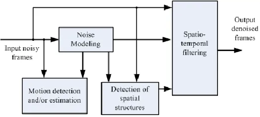
Fig. 1. General video denoising framework.
ISSN 2347-4289
)
(
)
(
1L
e
X
L
X
P
LX L LX
)
(
)
(
L
e
e
L
x
P
x Le xL Lx
)
(
2
)
(
2 1 2L
e
L
X
X
P
LX L L X
)
(
)
(
)
(
2 1L
L
L
X
E
X
var(
X
)
1
E
2(
X
)
denoising. We applied the same concept for denoising the video signals as was proposed for SAR image denoising. This paper is organized as follows. In the next sections the available literatures on multiplicative noise models have been reviewed. Section II provides a brief review of the filtering approach and describes the expressions for pdf of the noise models. An adaptive filtering recipe and its implementation details are described in Section III. Finally, simulation results to assess the effectiveness among the methods are presented in Section IV, whereas some conclusions are drawn in Section V.
2
L
ITERATURER
EVIEWA
NDT
HEORIESBilateral filter is a widely used nonlinear filter [10]-[12] introduced by Tomasi and Manduchi [10] which smoothes an image while preserving the edges. This filter replaces each pixel by weighted mean of nearby pixels considering both geometrical and photometrical distance using the domain and range filters. However, in [10], the corresponding domain and range filter parameters are set rather arbitrarily from image to image at different noise levels. For SAR image despeckling with bilateral filter, a limited number of approaches have been reported in the literature for adapting the parameters [11]- [12]. Adaptation of the parameters has been performed in [12] based on Equivalent Number of Looks (ENL) and the Edge Save Index (ESI). But the method takes the parameters in a nonadaptive and approximate basis in the iterative bilateral filtering steps and is also time consuming requiring ten iterations of filtering for each parameter estimation in the initial step. The method in [10] adapts the domain parameter using local Coefficient of Variation. However, it accounts photometrical similarity from a joint probability density function based model rather than utilizing the conventional range filter of the bilateral filtering framework. Hence, adaptation of range parameter is disregarded in [13]. However, the range parameter is more sensitive to noise compared to the domain parameter and thus entails its adaptation with underlying noise [11]. Recently, a bilateral filter is introduced to despeckle SAR images with an adaptive estimation of both filter parameters. The range parameter is tuned according to estimated noise level in SAR image implementing the Intensity Homogeneity Measurements based noise estimation method of [14]. Furthermore, domain parameter (d) has been adjusted
according to Coefficient of Variation that takes into account the local homogeneity of center to neighbouring pixels [13]. An iterative scheme is employed with adaptively estimated parameters in each iteration and the continuation of this process is determined from comparative difference in Structural Similarity Index (SSIM) [11]. Extensive simulations have been carried out to investigate their effectiveness and results have been reported for the noisy video signals’ frames. The results are compared among five available multiplicative natured noise models filtering methods.
2.1 Intensity Format
In coherent imaging system the images use electromagnetic waves which are backscattered from the targeted object. Con-sidering this, the frames are considered in two formats. One is in intensity format and the other one is in amplitude format. Let
Y
,X
andN
denote the image intensity, backscattering coefficient and normalized fading random variable in the noisy video frame respectively. The noise corrupted image can be considered as
Y
X
N
(1)where
Y
is in intensity format.The pdf of
X
is given by [15],
X
0
,
L
1
(2)where
L
denotes look (independent pixels) and
(
)
denotes gamma function. After taking natural logarithmic transformation (1) becomes
y
x
n
(3)where
y
ln(
Y
)
,x
ln(
X
)
andn
ln(
N
)
The transformation leads to a new pdf [15]-
(4)
The mean and variance of
P
x(
x
)
are given by
E
x(
x
)
(
L
)
ln(
L
)
(5)and
)
,
1
(
)
var(
x
L
(6)where
(
)
is digamma function and
(
1
,
L
)
is the first orderpolygamma function of
L
. Besides this, we could also pre-sume these frames asL
look images by taking square root operation. The pdf of which are also given here for the readers but this was beyond the scope of our focus and could be found elsewhere later on. It is clearly demonstrated that for intensity data log-transformed noise approaches Gaussian pdf faster than that of the original speckle [16].,
X
0
(7)The mean and variance are [15]
, (8)
After logarithmic the pdf, mean and variance become
x
Lx L x
Le
L
e
L
x
P
2 2exp
)
(
2
)
(
(9)
(
)
ln(
)
2
1
)
(
x
L
L
E
x
,(
1
,
)
4
1
)
] , [ [ , ] 2 ) ( ) ( 2 ) ( ) ( ] , [ [ , ] 2 2)
(
)
(
w wi i ww
j I i I j i j I i I j i w w
i i ww
d r d r d
e
e
j
I
i
I
2 1 1)
,
(
W
j
i
I
W i W j kl
2 1 1 2 2)
,
(
W
j
i
I
W i W j kl kl
) (1
)
(
d d Cov CK d
e
FA
Cov
)
(
)
(
)
(
i
M
i
V
i
Cov
L
C
d
0
.
714
L
K
W d7
.
0
ln
21
T
n
S
n
S
n
S
100
)
(
)
(
)
1
(
2.2 Amplitude Format
In amplitude format the multiplicative model is also represented by (1). For a single look image the normalized Rayleigh distributed random variable is [15]
4
exp
2
)
(
2X
X
X
P
X
,X
0
,
L
1
(11)The mean and the variance are [15]
1
)
(
X
E
X ,1
4
)
var(
X
(12)After taking logarithmic transform the statistics becomes Fisher-Tippet density function and is represented by-
4
exp
2
)
(
22x x
x
e
e
x
P
,L
1
(13)For the case of multilook the mean will be always be unity and the variance will be decreased by a factor of
L
.3 A
DAPTIVEB
ILATERALF
ILTERING OF THEV
IDEOF
RAMESThe bilateral filter replaces every pixel by a weighted sum of neighboring pixels. The weights depend on both the spatial distance and the photometric similarity. The output of the bila-teral filter is expressed as
(14)
where w is the span of the filter, indicating a window of size (2w+1)×(2w+1), and Id, I,d,r denote the denoised frames,
noisy frames, domain and range parameters respectively. Among the two filtering parameters, d is relatively insensitive
to noise variations [12]. As the main purpose of denoising is to reduce noise and r is more sensitive to noise variations, it is
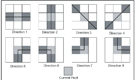
adaptively estimated in this method. Let Skl denote a W×
W-sized block centered on the (k, l)-th pixel. The homogeneity of the block is measured along eight directions as shown in Fig. 2. For a given direction, a weighted sum of the corresponding pixels gives the homogeneity measure in that direction, the weights assigned for a block being
1,
1,..,
(W
1),..,
1,
1
.Fig. 2. Directions of the homogeneity measurement for a 3×3 block.
Assuming the pixels in a block to be independent and identi-cally distributed (i.i.d.), the corresponding mean and variance, denoted by µkl and kl2, respectively, are computed as
(15)
(16)
where I(i, j) represents the (i, j)-th pixel of a noisy frame. Since the domain parameter is related to spatial closeness of pixels, it is adapted according to Coefficient of Variation (Cov). d is
related to Cov according to the following formula [13]
(17)
Where
, , (18)
where V(i) and M(i) are the variance and mean of pixels in the local window, A, Kd, and Cd are parameters determining the
upper limit, the decay speed, and the symmetry center of d as
a function of Cov , respectively with a factor F=0.3. The bila-teral filtering operation is performed in an iterative manner in this method. The purpose of having iteration is to reduce the residual noise through repeated filtering. After each iteration, the parameters are estimated from the resultant denoised frame. As repeated filtering may lead to the removal of frame structures with noise, using the percentage difference in the structural similarity index (SSIM) [17] obtained at the n-th and n+1-th iteration, a stopping criterion is defined as
(19)
be-ISSN 2347-4289
tween the SSIM of the noisy frame from the two consecutive iterations reaches at the threshold T = 5, the two filtered frames are nearly similar. Hence, the filtering process is stopped since further filtering may lead to blurring of the edges, removal of frame structure with noise etc.
4 S
IMULATIONR
ESULTSThree Additive White Gaussian Noise (AWGN) corrupted vid-eos namely, gflowersg15.avi (flower garden), gsales-mang15.avi (salesman) and gstennisg15.avi (tennis player [18] are used for extensive simulations. Each one contains 50 frames. The pdf of the noise models are considered in ampli-tude format. Simulations were carried out by considering mul-tiplicative noise nature as are used for denoising the speckle noises of the SAR images. For the Bayes-shrink [13], five level decomposition is carried out with the Daubechies’ wavelet of order 8. The ENL and ESL based adaptive bilateral in [19] was initialized with d = 3 and r = 0.05 with a step size of 0.05.
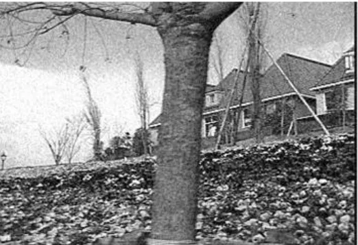
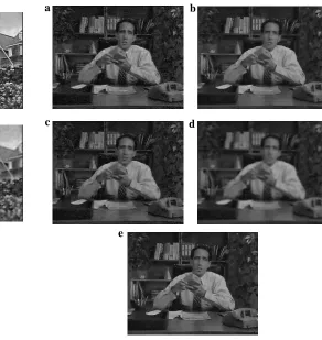
Table I, II and III show the average value of PSNR(dB), struc-tural similarity index (SSIM) and edge preservation index (β) of the video frames. Although from a PSNR point of view our method is not always significantly better than the other me-thods, it invariably performs best visually as can be seen in Figs. 4, 6 and 8. Three noisy frames are shown in Fig. 3, 5 and 7 to compare with the corresponding denoised frames. Amongst these filters Frost performs the worst in terms of vis-ual qvis-uality in terms of spatio-temporal blur. The visvis-ual qvis-uality of Bayes-Shrink, Bilateral, Adaptive Bilateral and ENL Bilateral is nearly same. The standard deviation of PSNR, SSIM and β of the methods are obtained as 1.42, 0.08 and 0.046 respec-tively except the Frost filter.
TABLE I. FLOWER GARDEN (gflowersg15.avi)
Method PSNR(dB) SSIM β
Bayes-Shrink 25.51141 0.800954 0.898216 Bilateral 25.62475 0.788338 0.936662 Adaptive
Bila-teral
25.55384 0.764352 0.905316
Frost 16.9392 0.3895 0.41486 ENL Bilateral 22.7178 0.6274 0.828694
TABLE II. SALESMAN (gsalesmang15.avi)
Method PSNR(dB) SSIM β Bayes-Shrink 24.91301 0.67457 0.5962 Bilateral 25.88039 0.653032 0.833696 Adaptive
Bila-teral
25.03207 0.641336 0.674246
Frost 22.15655 0.338266 0.218848 ENL Bilateral 25.70528 0.604316 0.65549
TABLE III. TENNIS PLAYER (gstennisg15.avi)
Method PSNR(dB) SSIM β
Bayes-Shrink 24.0291 0.522752 0.627794 Bilateral 25.20242 0.601848 0.814058 Adaptive
Bila-teral
24.13672 0.50076 0.65928
Frost 20.68966 0.200206 0.219756 ENL Bilateral 24.52833 0.509458 0.686952
5 C
ONCLUSIONFor high-quality video denoising a real and structured noise model is essential. Simulation results show that the systems can play significant role with the state of the art in removing AWGN and structured noise. Robust motion estimation is es-sential for high-quality video denoising which be area for fur-ther investigation along with multiplicative noise model. In this paper, an adaptive bilateral filter has been introduced for video frames denoising. The method suppresses speckle noise well, while retaining the structure and edges of the frames. The do-main parameter is adjusted according to Coefficient of Va-riance of local neighborhood. The range parameter is adapted with present spackle noise in the frames which are estimated from Intensity Homogeneity Measurements of the frames. The method outperforms all the other methods regarding objective and subjective criteria such as, PSNR, SSIM, edge preserva-tion index as well as in terms of visual quality of the frames.
a
b
c
d
e
Fig. 4. Denoised frame of Flower Garden (10-th frame). (a) Bayes-Shrink (b) Bilateral (c) Adaptive Bilateral (d) Frost (e)
ENL Bilateral.
Fig. 5. Noisy frame of Salesman (10-th frame).
a b
c d
e
Fig. 6. Denoised frame of Salesman (10-th frame). (a) Bayes-Shrink (b) Bilateral (c) Adaptive Bilateral (d) Frost (e) ENL
Bila-teral.
ISSN 2347-4289
a
c
b
d
e
Fig.8. Denoised frame of Tennis Player (10-th frame). (a) Bayes-Shrink (b) Bilateral (c) Adaptive Bilateral (d) Frost (e)
ENL Bilateral. .
A
CKNOWLEDGMENTThe authors would like to acknowledge Department of Elec-trical and Electronic Engineering, Ahsanullah university of Science and Technology for conducting the research reported in the paper.
R
EFERENCES[1] C. Liu and W. T. Freeman, “A High-Quality Video Denoising Algorithm Based on Reliable Motion Estimation.” Computer Vision – ECCV 2010. Ed. Kostas Daniilidis, Petros Maragos, & Nikos Paragios. LNCS Vol. 6313. Berlin, Heidelberg: Springer Berlin Heidelberg, 2010, pp.706–719.
[2] P. Moulin and J. Liu, “Analysis of multiresolution image denoising schemes using generalized Gaussian and complexity priors,” IEEE Trans. on Info. Theory, Vol. 45, No. 3, 1999, pp.909-919.
[3] M. Maggioni, G. Boracchi, A. Foi and K. Egiazarian, “Video Denoising, Deblocking, and Enhancement Through Separable 4-D Nonlocal Spatiotemporal Transforms,” , IEEE Trans. on Image Process., Vol. 21, No. 9, 2012, pp.3952 - 3966.
[4] A. Amer and E. Dubois, “Fast and reliable structure-oriented video noise estimation,” IEEE Trans. on Circuits and Systems for Video Technology, Vol. 15, No. 1, 2005, pp.113–118.
[5] H. Cheong, A. Tourapis, J. Llach and J. Boyce, “Adaptive spatio-temporal filtering for video de-noising,” IEEE, Inter. Conf. on Image Process., 2004, pp.965–968.
[6] G. de Haan, P. Biezen, H. Huijgen, and O. Ojo, “True-motion estimation with 3-d recursive search block matching,” IEEE Trans. on Circuits and Systems for Video Technology, Vol. 3, No. 5, 1993, pp.368–379
.
[7] J. S. Lee, “Speckle analysis and smoothing of synthetic aperture radar images,” Comput. Graph. Image Process., Vol-17, 1981, pp.24-32.
[8] J. A. Stiles, K. S. Shanumugan, and J. C. Holtzman, “A model for radar images and its application to adaptive digital filtering of multiplicative noise,” IEEE Trans. Pattern Anal. Mach. Intell., Vol. 4, No. 2, 1986, pp. 157-165.
[9] V. Zlokolica, "Advanced Nonlinear Methods for Video Denoising," PhD Thesis, Faculteit Ingenieurswetenschappen Academiejaar, 2005-2006, Universiteit Gent.
[10]C. Tomasi and R. Manduchi, “Bilateral filtering for gray and color images,” IEEE Inter. Conf. on Comp. Vision, 1998, pp.839–846.
[11]M. Zhang and B. K. Gunturk, “Multiresolution bilateral filtering for image denoising,” IEEE Trans. on Image Process., Vol. 17, No. 12, 2008, pp. 2324–2332.
[12]W. G. Zhang, F. Liu and L. C. Jiao, “SAR image despeckling via bilateral filtering,” IET Electronics Letters, Vol. 45, No. 15, 2009, pp.781-783.
[13]G. Ting Li, C. Le Wang, P. Ping Huang and W. Dong Yu, “SAR Image Despeckling Using a Space-Domain Filter With Alterable Window”, IEEE Geo. and Remote Sensing Let., Vol. 10, No. 2, 2012, pp.263-267.
[14]A. Amer and E. Dubois, “Fast and Reliable Structure-Oriented Video Noise Estimation,” IEEE Trans. on Circuits and Systems for Video Tech., Vol. 15, No. 1, 2005, pp.113-118.
[15]F. Ulaby and M. C. Dobson, “Handbook of Radar Scattering Statistics for Terrain. Norwood,” MA: Artech House, 1989.
[16]H. Xie, L. E. Pierce, and F. T. Ulaby, “Statistical Properties of Logarithmically Transformed Speckle,” IEEE Trans. on Geo. and remote sensing, Vol. 40, No. 3, 2002, pp.721-727.
[17]Z. Wang, A. C. Bovik, H. R. Sheikh and E. P. Simoncelli,“Image quality assessment: from error visibility to structural similarity,” IEEE Trans. on Image Process., Vol. 13, No. 4, 2004, pp. 600-612.
[18]http://telin.ugent.be/~vzlokoli/Results_J/noisy/