Article
A Recursive Wheel Wear and Vehicle Dynamic
Performance Evolution Computational Model for Rail
Vehicles with Tread Brakes
Smitirupa Pradhan and Arun Kumar Samantaray *
Center for Railway Research (CRR-IIT Kharagpur), Department of Mechanical Engineering, Indian Institute of Technology (IIT), Kharagpur 721302, India; [email protected]
* Correspondence: [email protected]
Received: 22 March 2019; Accepted: 11 April 2019; Published: 17 April 2019 Abstract:The increased temperature of the rail wheels due to tread braking causes changes in the wheel material properties. This article considers the dynamic wheel material properties in a wheel wear evolution model by synergistically combining a multi-body dynamics vehicle model with a finite element heat transfer model. The brake power is estimated from the rail-wheel contact parameters obtained from vehicle model and used in a finite element model to estimate the average wheel temperature. The wheel temperature is then used for wheel wear computation and the worn wheel profile is fed to the vehicle model, thereby forming a recursive simulation chain. It is found that at a higher temperature, the softening of the rail-wheel material increases the rate of wheel wear. The most affected dynamic performance parameter of the vehicle is found to be the critical speed, which reduces sharply as the wheel wear exceeds a critical limit.
Keywords: tread braking; wheel-rail contact; tread wear; vehicle dynamics
1. Introduction
Several types of braking systems are used in railway vehicles. Tread braking along with electro-dynamic/disc braking is frequently used in freight, and low-speed suburban and metro trains due to its lower manufacturing cost, simple structure and ease of control. During tread braking, brake shoes/blocks press against the wheel tread and frictional heat is generated both at the wheel–brake block and wheel–rail interfaces. The heat generated due to braking is shared by the wheel, rail and block through thermal resistances and heat capacities [1]. Some amount of heat is also transferred into the surrounding through convection and radiation. Due to thermo–mechanical interaction, hot spots are often found on the wheel tread [2,3]. The amount of heat transfer between two contact-surfaces can be explained by the concept of third body approach [4], where wear debris, contaminants, sand, lubricant and leaves, etc. represent the third body.
There is a wide range of literature which contains both numerical approaches and experimental studies to understand the concept of heat transfer between the wheel-rail and wheel-block interfaces. The temperature rise due to slip at the wheel-rail interface has been studied by Tanvir [5]. Knothe and Liebelt [6] have studied the contact temperature at the wheel–rail contact surface due to sliding motion, where they have reduced a three-dimensional problem to a two-dimensional one, as an approximation. Furthermore, they have evaluated the effect of roughness and surface defect on the temperature distribution.
Ertz and Knothe [7] have calculated the temperature distribution on the wheel due to rolling along with sliding friction and concluded that the temperature rise due to braking is confined within a very thin layer near the contact surface. Among other notable works, Ma et al. [8] studied the tribological
responses on the surface and sub-surface of the wheel-rail interface for different operating conditions, Tudor et al. [9] developed an analytical solution for the temperature distribution at the wheel–rail and wheel–brake block contact surfaces, Spiryagin et al. [10] studied the temperature distribution at the wheel flange–rail head interface, Naeimi et al. [11] computed flash temperature and stress-strain responses, Chen and Wang [12] analyzed the thermo-mechanical behavior of elasto-plastic bodies to study the impact of sliding speed and thermal softening on the contact behavior, and Kennedy et al. [13] built a finite element (FE) model to estimate the temperature distribution and heat partition between wheel and rail. Moreover, the effect of thermal loading on the fatigue life of the wheel is studied in [14,15], on material deformation and damage in [16] and on the bearing life in [17].
Many researchers have focused on the temperature distribution on the wheel profile due to constant brake power which is not comparable to the actual operating conditions. In this article, variable brake power similar to the real operating conditions is considered. The temperature at the tread of the wheel can rise up to 550◦C and in some extreme cases, it can go up to 800 ◦C [18]. Sometimes, the temperature may rise approximately up to 1050◦C due to skidding and locking of the wheels along the rail for a short span of time, as shown in the experimental results [19,20]. This causes phase transformations in the steel and leads to spall formation or wheel flat. Moreover, due to thermal loading, plastic deformation takes place and the microstructure on the wheel−tread surface changes. However, the aforementioned case is beyond the scope of the current research work. The accompanying thermal stresses and thermal softening due to elevated temperature increase the wheel wear rate. At higher temperature, the influence of thermal softening on wear rate is more pronounced than thermal stresses [21]. When the temperature due to braking is in the range of 300−350◦C, the wheel is more resistant to fatigue due to strain hardening [22].
Depending upon the operating conditions, single or multi point contact patches [23] occur at the tread and tread-flange. To calculate wear distribution, it is necessary to know the location of the contact patch, slip between the wheel and rail and the contact forces. Several researchers have suggested a number of approaches to predict the wear distribution in the wheels of the railway vehicles. The consequences of the worn wheel on the dynamics of the vehicle (such as creep force, creepage, critical and derailment speeds as well as change of size and location of the contact patches) are analyzed in limited literature, though its heavy wear is known to be detrimental to vehicle performance. Therefore, friction modifiers [24] are often used in tracks.
Although, the wheel and rail surfaces are rough due to wear, for simplifying the problem, it is assumed that the surfaces are smooth. Archard [25] has shown that the surface roughness has negligible effect on heat conduction. Several researchers focused on the estimation of the wear distribution due to braking [26,27]. In [26], disc brakes are used in the wheels and hence, the thermal influence on wheel/rail material properties is neglected. A very limited work has been reported on the wear distribution by considering the effect of wheel temperature during tread braking.
Vehicles2019,1 90
2. Materials and Methods
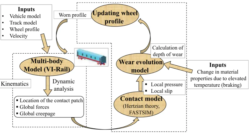
The objective of this study is to develop a wear evolution model by considering the influence of temperature on the wheel material due to tread braking. The schematic representation of the recursive wheel wear and vehicle dynamics evolution process is shown in Figure1. This tool deals with the estimation of wear distribution at the wheel surface under realistic vehicle operation by considering the change in material properties at the elevated temperature. During running, the vehicle accelerates, decelerates (including slowing before the curves and stop braking) and moves at constant velocity (intermediate cooling period). The temperature change in the brake block-wheel-rail system is estimated as per the vehicle operating condition. The model is composed of three interactive interfaces, namely the vehicle model, thermal model and wear model. The vehicle model is built in commercial multi-body simulation (MBS) software, VI-RailTMin which dynamic simulation is performed. The outputs such as creepage (lateral, longitudinal and spin), instantaneous rolling radius, location of the contact patch, creep forces, etc. are collected from post-processing of the results from the dynamic simulation. Creep forces and creepages as per the specified vehicle speed profile are then used to calculate the brake power at the blocks and the contact patch on the rail. The thermal model is developed by using FE approach where heat fluxes corresponding to the brake power are generated at the brake blocks and the contact patch on the rail. The temperature field is found from this analysis and the corresponding changes in the physical properties of the wheel material at the tread surface are determined by mapping those to the available experimental data. The changes in material properties and the vehicle dynamics simulation results (creepages, contact patch location and dimension, etc.) are then used in a MATLAB®program for calculating the wear distribution on the wheel surface. The worn wheel profile is then generated and used recursively for further dynamic analysis.
2019, 1, 6 90
The objective of this study is to develop a wear evolution model by considering the influence of temperature on the wheel material due to tread braking. The schematic representation of the recursive wheel wear and vehicle dynamics evolution process is shown in Figure 1. This tool deals with the estimation of wear distribution at the wheel surface under realistic vehicle operation by considering the change in material properties at the elevated temperature. During running, the vehicle accelerates, decelerates (including slowing before the curves and stop braking) and moves at constant velocity (intermediate cooling period). The temperature change in the brake block-wheel-rail system is estimated as per the vehicle operating condition. The model is composed of three interactive interfaces, namely the vehicle model, thermal model and wear model. The vehicle model is built in commercial multi-body simulation (MBS) software, VI-RailTM in which dynamic simulation is performed. The outputs such as creepage (lateral, longitudinal and spin), instantaneous rolling radius, location of the contact patch, creep forces, etc. are collected from post-processing of the results from the dynamic simulation. Creep forces and creepages as per the specified vehicle speed profile are then used to calculate the brake power at the blocks and the contact patch on the rail. The thermal model is developed by using FE approach where heat fluxes corresponding to the brake power are generated at the brake blocks and the contact patch on the rail. The temperature field is found from this analysis and the corresponding changes in the physical properties of the wheel material at the tread surface are determined by mapping those to the available experimental data. The changes in material properties and the vehicle dynamics simulation results (creepages, contact patch location and dimension, etc.) are then used in a MATLAB® program for calculating the wear distribution on the wheel surface. The worn wheel profile is then generated and used recursively for further dynamic analysis.
Contact model
(Hertzian theory, FASTSIM)
Wear evolution
model
Updating wheel
profile
Calculation of depth of wear
Local pressure
Local slip
Multi-body
Model (VI-Rail)
Location of the contact patch
Global forces
Global creepage
Dynamic
analysis
Kinematics
Inputs
• Vehicle model • Track model • Wheel profile • Velocity
Inputs
Change in material properties due to elevated
temperature (braking) Worn profile
Figure 1. Architecture of recursive simulation model.
During the above-mentioned procedure, the main assumptions made to simplify the model are as follows:
• Wear in the rail is much less as compared to that in the wheel and hence is not taken into account.
• The contact between wheel and rail is in dry condition and the presence of a third body (worn particles of wheel, rail and block, water, sand and leaves) is not considered.
• The rail-wheel contact patch is elliptical in shape and the contact patch lies in the wheel tread, which is far away from the flange root.
• There is no wear in flange due to small duration, intermittent secondary contacts at entry and exit curves.
• The wheel and rail materials are same and have similar hardness. Figure 1.Architecture of recursive simulation model.
During the above-mentioned procedure, the main assumptions made to simplify the model are as follows:
• Wear in the rail is much less as compared to that in the wheel and hence is not taken into account. • The contact between wheel and rail is in dry condition and the presence of a third body (worn
particles of wheel, rail and block, water, sand and leaves) is not considered.
• There is no wear in flange due to small duration, intermittent secondary contacts at entry and exit curves.
• The wheel and rail materials are same and have similar hardness.
• The wheel and rail material are isotropic, i.e., the material properties are same in all directions at a point but can vary from point to point due to change in temperature.
• The brake pad/shoe is made up of softer material (usually composite material with modulus of elasticity about ten times less as compared to wheel-rail material) and hence there is no wheel wear (but brake shoe/pad wear) at brake pad and wheel contact.
• The brake pads are assumed to be replaced periodically to maintain conformal contact between the brake pad and wheel tread, and the contact pressure between the wheel and brake pad is uniform. • The heat partition between the wheel-rail-brake block is not influenced by the wheel wear. • The influence of rail temperature variation is neglected in the model because it is usually much
smaller than wheel temperature variation. Rail temperature is assumed to remain constant at 30◦
C.
• Plastic deformation and fatigue effects are not considered.
• Spall formation, wheel flat etc. induced by phase transformation of the wheel and rail material at high contact pressure and temperature is neglected. The average contact patch pressure and temperature are considered for estimating the material properties while neglecting the local variations within the contact patch.
3. Wear Prediction Tool 3.1. Vehicle Model
An ERRI wagon/vehicle (Figure2) with one coach and two bogies (front and rear) is used as a standard model for our research. The important components of the bogie are wheel (profile is s1002), secondary suspension system (air spring, secondary lateral and vertical dampers, anti-yaw damper and bump-stops) and the primary suspension system consists of axle box, helical spring and primary vertical damper as shown in Figure2. The parametric values of the important components of the bogie are given in Table1.
2019, 1, 6 91
• The wheel and rail material are isotropic, i.e., the material properties are same in all directions at a point but can vary from point to point due to change in temperature.
• The brake pad/shoe is made up of softer material (usually composite material with modulus of elasticity about ten times less as compared to wheel-rail material) and hence there is no wheel wear (but brake shoe/pad wear) at brake pad and wheel contact.
• The brake pads are assumed to be replaced periodically to maintain conformal contact between the brake pad and wheel tread, and the contact pressure between the wheel and brake pad is uniform.
• The heat partition between the wheel-rail-brake block is not influenced by the wheel wear. • The influence of rail temperature variation is neglected in the model because it is usually
much smaller than wheel temperature variation. Rail temperature is assumed to remain constant at 30oC.
• Plastic deformation and fatigue effects are not considered.
• Spall formation, wheel flat etc. induced by phase transformation of the wheel and rail material at high contact pressure and temperature is neglected. The average contact patch pressure and temperature are considered for estimating the material properties while neglecting the local variations within the contact patch.
3. Wear Prediction Tool
3.1. Vehicle Model
An ERRI wagon/vehicle (Figure 2) with one coach and two bogies (front and rear) is used as a standard model for our research. The important components of the bogie are wheel (profile is s1002), secondary suspension system (air spring, secondary lateral and vertical dampers, anti-yaw damper and bump-stops) and the primary suspension system consists of axle box, helical spring and primary vertical damper as shown in Figure 2. The parametric values of the important components of the bogie are given in Table 1.
Axle box Air spring
Secondary vertical damper Secondary lateral damper
Primary vertical damper Primary suspension
Anti yaw damper
y
x z
(b) (a)
Figure 2. Important bogie components and (b) Full vehicle model (two bogies with car body).
In Table 1, Kx, Ky and Kz are the stiffnesses of the primary suspension in x, y and z directions, respectively, Kθand Kα are the torsional stiffnesses in x and y directions, respectively. All the dampers are designed with nonlinear damping and series stiffness (standard data for ERRI bogie available in VI-RAIL). The standard ERRI bogie and coach parameters are considered (except primary suspension system) with air spring. To attain stability against hunting in a straight track, higher longitudinal and lateral stiffness of the primary suspension is required.
3.2. Track Model
Generally, flexible track is modeled separately in the VI-rail which is also the input parameter to the multi-body model for dynamic analysis. For the dynamic and thermal analysis, a flexible railway track between two Indian cities, Bhubaneswar and Cuttack of length 27.9 km has been considered (more details are given in [26]). This track comprises 69.4% straight, 14.9% transition and
Vehicles2019,1 92
Table 1.Parameter values of important components of vehicle [26].
Parameters of MBS Model Parameter Values Quantity
Mass of car body MCB=32,000 kg 1
Rotary inertias of car body
Ixx=5.68×10⁴kg m2
Iyy=1.97×10⁶kg m2
Izz=1.97×10⁶kg m2
Mass of Bogie frame Mbogie=2615 kg 2
Rotary inertias of bogie frame
Ixx=1722 kg m2
Iyy=1476 kg m2
Izz=3067 kg m2
Mass of Wheel-set Mwheel=1503 kg 4
Rotary inertias of wheel-set
Ixx=810 kg m2
Iyy=810 kg m2
Izz=112 kg m2
Mass of Axle-box Mabox=155 kg 8
Rotary inertias of axle box
Ixx=2.1 kg m2
Iyy=5.6 kg m2
Izz=5.6 kg m2
Stiffness of Primary suspension
Kx=6.8×10⁶N/m
8
Ky=3.92×10⁶N/m
Kz=5.756×10⁵N/m
Kθ=Kα=63.5 Nm/rad
Nominal pressure of Secondary suspension (Air spring) Pstatic=2.0532×10⁵Pa 4 Primary vertical damper (series stiffness) 1.0×10⁶N/m 8 Secondary vertical damper (series stiffness) 6.0×10⁶N/m 4
Secondary anti-yaw damper (series stiffness) 3.0×10⁷N/m 4 Secondary lateral damping (series stiffness) 6.0×10⁶N/m 4
In Table1,Kx,KyandKzare the stiffnesses of the primary suspension inx,yandzdirections, respectively,KθandKαare the torsional stiffnesses inxandydirections, respectively. All the dampers are designed with nonlinear damping and series stiffness (standard data for ERRI bogie available in VI-RAIL). The standard ERRI bogie and coach parameters are considered (except primary suspension system) with air spring. To attain stability against hunting in a straight track, higher longitudinal and lateral stiffness of the primary suspension is required.
3.2. Track Model
Vehicles2019,1 93 15.65% curved portions as shown in Figure 3. The track design parameters are curvature, cant/super-elevation, transition curve, rail inclination, gauge and rail profile (UIC 60) and rail materials (Young modulus, Poisson’s ratio), etc. The considered track consists of both small (smallest 526.3 m) and medium (largest 2000 m) curves. For estimation of critical speed and derailment speed, ramp type irregularities (width 5 mm and height 5 mm) are used.
Table 1. Parameter values of important components of vehicle [26].
Parameters of MBS model Parameter values Quantity
Mass of car body MCB = 32,000 kg 1
Rotary inertias of car body Ixx= 5.68 × 10⁴ kg m2 Iyy= 1.97 × 10⁶ kg m2 Izz= 1.97 × 10⁶ kg m2
Mass of Bogie frame Mbogie = 2,615 kg 2
Rotary inertias of bogie frame Ixx= 1,722 kg m2 Iyy= 1,476 kg m2 Izz= 3,067 kg m2
Mass of Wheel-set Mwheel = 1,503 kg 4
Rotary inertias of wheel-set Ixx= 810 kg m2 Iyy= 810 kg m2 Izz= 112 kg m2
Mass of Axle-box Mabox = 155 kg 8
Rotary inertias of axle box Ixx= 2.1 kg m2
Iyy= 5.6 kg m2
Izz= 5.6 kg m2
Stiffness of Primary suspension Kx = 6.8 × 10⁶ N/m Ky = 3.92 × 10⁶ N/m Kz = 5.756 × 10⁵ N/m Kθ = Kα = 63.5 Nm/rad
8
Nominal pressure of Secondary suspension (Air spring) Pstatic = 2.0532 × 10⁵ Pa 4
Primary vertical damper (series stiffness) 1.0 × 10⁶ N/m 8
Secondary vertical damper (series stiffness) 6.0 × 10⁶ N/m 4
Secondary anti-yaw damper (series stiffness) 3.0 × 10⁷ N/m 4
Secondary lateral damping (series stiffness) 6.0 × 10⁶ N/m 4
L
2
L
1 L
3
L
11
L
12
L
15
L
22
L
25
Figure 3. Track between two Indian cities Bhubaneswar and Cuttack at distance 27.9 km [26].
3.3. Thermal Model
Figure 3.Track between two Indian cities Bhubaneswar and Cuttack at distance 27.9 km [26].
3.3. Thermal Model
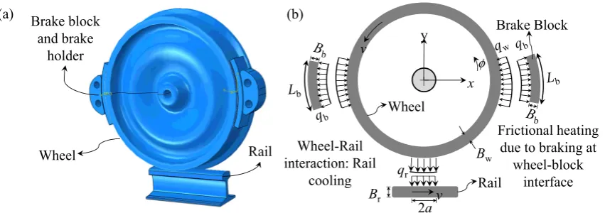
Most of the railway vehicles in India employ mechanical braking such as tread braking and axle mounted disc braking. In tread braking, brake blocks/shoes directly come into contact with the tread of the wheel to stop and/or decelerate the vehicle. Depending on the application, different types such as clasp and tandem block arrangements (One/two block/s per wheel) are used. In this paper, two blocks per wheel and clasp arrangement (Figure4a) is used for the analysis. Heat is generated due to friction at the brake shoe and moving tread interface and heat is transferred into the wheel and rail along with the brake shoe (as shown in Figure4b). The part of heat transferred to the wheel (heat partition factor) depends on total contact area, total heat capacity of blocks and cooling conditions (as shown in Figure4b), which is calculated as [28,29].
β=
1+ κw
κb !1/2
λb
λw
Ab Aw
−1
(1)
Here,Ais the area in contact,κis thermal diffusivity,λis thermal conductivity, subscripts b and w stand for brake block and wheel, respectively. The part of total heat transferred into the block is expressed as (1−β). After calculating the heat partition factor, the thermal analysis is straightforward with known brake power/heat fluxes at the contact surfaces.
The dimensionless Peclet number is Pe=aV/2κ, whereais semi-axis length of the contact patch in the rolling direction,Vis the peripheral velocity of the wheel with thermal diffusivityκ=λ/ρCp which depends on thermal conductivity, mass density (ρ) and specific heat capacity of the material (Cp). Pe helps to determine the type (1D/2D/3D) of heat conduction. In this paper, the minimum velocity is 16.8 m/s except stop braking, the size ofavaries from 4.9 mm to 7.2 mm as the velocity varies with time. The thermal diffusivity for steel isκ=14.2×10⁻⁶m2/s [7]. The minimum estimated value of Pe is 5797 except during stop braking, which determines that the heat conduction occurs only normal to the contact plane, i.e., inz-direction as Pe>10 [30]. Therefore, by neglecting longitudinal and lateral heat conduction (xandydirection), the one-dimensional heat conduction equation is given by
κ∂2T
∂z2 =
∂T
∂t (2)
Vehicles2019,1 94
2019, 1, 6 93
Most of the railway vehicles in India employ mechanical braking such as tread braking and axle mounted disc braking. In tread braking, brake blocks/shoes directly come into contact with the tread of the wheel to stop and/or decelerate the vehicle. Depending on the application, different types such as clasp and tandem block arrangements (One/two block/s per wheel) are used. In this paper, two blocks per wheel and clasp arrangement (Figure 4a) is used for the analysis. Heat is generated due to friction at the brake shoe and moving tread interface and heat is transferred into the wheel and rail along with the brake shoe (as shown in Figure 4b). The part of heat transferred to the wheel (heat partition factor) depends on total contact area, total heat capacity of blocks and cooling conditions (as shown in Figure 4b), which is calculated as [28,29].
1 1 2
w b b
b w w
1 A A
κ
λ
β
κ
λ
− = + (1)Here, A is the area in contact, κ is thermal diffusivity, λ is thermal conductivity, subscripts b and w stand for brake block and wheel, respectively. The part of total heat transferred into the block is expressed as (1 − β). After calculating the heat partition factor, the thermal analysis is straightforward with known brake power/heat fluxes at the contact surfaces.
The dimensionless Peclet number is Pe=aV 2κ, where a is semi-axis length of the contact patch in the rolling direction, V is the peripheral velocity of the wheel with thermal diffusivity
p
C
κ λ ρ= which depends on thermal conductivity, mass density (
ρ
) and specific heat capacity of the material (Cp). Pe helps to determine the type (1D/2D/3D) of heat conduction. In this paper, the minimum velocity is 16.8 m/s except stop braking, the size of a varies from 4.9 mm to 7.2 mm as the velocity varies with time. The thermal diffusivity for steel isκ
=14.2 10× −6m2/s [7]. The minimum estimated value of Pe is 5,797 except during stop braking, which determines that the heat conduction occurs only normal to the contact plane, i.e., in z-direction as Pe > 10 [30]. Therefore, by neglecting longitudinal and lateral heat conduction (x and y direction), the one-dimensional heat conduction equation is given by2 2 T T t z κ ∂ =∂ ∂ ∂ (2)
where T stands for the instantaneous temperature and t is the time.
Brake block and brake holder Rail Wheel v 2a Br Bw v qr y x φ Rail Wheel Brake Block Frictional heating due to braking at
wheel-block interface Wheel-Rail interaction: Rail cooling (a) (b)
Figure 4. (a) Wheel-brake block-rail assembly and (b) Schematic diagram of distribution of frictional heat fluxes (qw and qb) at block-wheel interface and cooling flux (qr) at wheel-rail interface.
The frictional power is generated during braking, which is converted into heat in the corresponding contact area (wheel–brake block and wheel–rail). To estimate the steady temperature, the commercial FE package, ABAQUS/Standard was used to model wheel–block–rail system (as shown in Figure 4a) which is a three-dimensional model. The block and block holder are modeled by FE approach as well. The mean heat flux over the brake block contact area is calculated as
Figure 4.(a) Wheel-brake block-rail assembly and (b) Schematic diagram of distribution of frictional heat fluxes (qwandqb) at block-wheel interface and cooling flux (qr) at wheel-rail interface.
The frictional power is generated during braking, which is converted into heat in the corresponding contact area (wheel–brake block and wheel–rail). To estimate the steady temperature, the commercial FE package, ABAQUS/Standard was used to model wheel–block–rail system (as shown in Figure4a) which is a three-dimensional model. The block and block holder are modeled by FE approach as well. The mean heat flux over the brake block contact area is calculated as
qbrake= Qbrake HbLb
(3)
whereQbrake is the thermal power generated during braking, block length (Lb) and block width (Hb) are 320 mm and 80 mm, respectively [31]. The amount of the brake power depends on the operating conditions of the vehicle. The vehicle reduces its velocity when it enters the transition and the curved portions of the track. Hence, the braking power varies according to the velocity profile as shown in Figure5. The transient heat transfer can be explained by a conduction–convection (convection-diffusion) equation, i.e.,
div(K∇T)
| {z }
Diffusion
=Cpρ
∂T/∂t+ ν.∇T |{z} Convection (4)
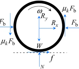
where div is the divergence vector operator,Kis the thermal conductivity matrix,∇refers to the vector differential operator andv=[vx(x,y),vy(x,y)]Tthe velocity vector of spatial points [31]. During the curving, the braking force (Fb) (as shown in Figure6, whereRxandRyare reactions at axle in thex andydirections, respectively) acting on the wheel due to braking (deceleration) and corresponding braking power is calculated.
2019, 1, 6 94
brake brake b b Q q H L = (3)
where Qbrake is the thermal power generated during braking, block length (Lb) and block width (Hb) are 320 mm and 80 mm, respectively [31]. The amount of the brake power depends on the operating conditions of the vehicle. The vehicle reduces its velocity when it enters the transition and the curved portions of the track. Hence, the braking power varies according to the velocity profile as shown in Figure 5. The transient heat transfer can be explained by a conduction–convection (convection-diffusion) equation, i.e.,
(
)
p Convection Diffusion
div ∇T =C ρ∂ ∂ + ∇T t . T
K ν (4)
where div is the divergence vector operator, K is the thermal conductivity matrix, ∇refers to the vector differential operator and v = [vx (x, y), vy (x, y)]T the velocity vector of spatial points [31]. During the curving, the braking force (Fb) (as shown in Figure 6, where Rx and Ry are reactions at axle in the x and y directions, respectively) acting on the wheel due to braking (deceleration) and corresponding braking power is calculated.
0 5 10 15 20 25
0 400 800 1200
Time (s) V eloci ty (m/ s)
Figure 5. Velocity profile for acceleration and braking.
ω
yR
xR
W
bF
b kF
μ
b kF
μ
bF
Nf
Figure 6. Calculation of brake force in curved track.
It is assumed that the power generated due to friction is dissipated as heat over the common contact area between block and wheel and total heat generated is partitioned between the wheel and block. By neglecting longitudinal rail gradient, buff and draft forces, etc. the power at the wheel-block interface during braking is estimated by solving
(
2 k b)
,J
θ
= −μ
F − f R (5)brake 2 k b for 0
P =
μ
F Rω
θ
< (6)where J is the polar moment of inertia of wheel and axle, R the mean radius of the wheel at nominal tread region, μk(μk= 0.2) the coefficient of kinematic friction (full slip) brake block-wheel interface, f
Vehicles2019,1 95
brake brake
b b Q q
H L
= (3)
where Qbrake is the thermal power generated during braking, block length (Lb) and block width (Hb) are 320 mm and 80 mm, respectively [31]. The amount of the brake power depends on the operating conditions of the vehicle. The vehicle reduces its velocity when it enters the transition and the curved portions of the track. Hence, the braking power varies according to the velocity profile as shown in Figure 5. The transient heat transfer can be explained by a conduction–convection (convection-diffusion) equation, i.e.,
(
)
p Convection Diffusion
div ∇T =C ρ∂ ∂ + ∇T t . T
K ν (4)
where div is the divergence vector operator, K is the thermal conductivity matrix, ∇refers to the vector differential operator and v = [vx (x, y), vy (x, y)]T the velocity vector of spatial points [31]. During the curving, the braking force (Fb) (as shown in Figure 6, where Rx and Ry are reactions at axle in the x and y directions, respectively) acting on the wheel due to braking (deceleration) and corresponding braking power is calculated.
0 5 10 15 20 25
0 400 800 1200
Time (s)
V
eloci
ty
(m/
s)
Figure 5. Velocity profile for acceleration and braking.
ω
y
R
x
R
W
b
F
b
k
F
μ
b
k
F
μ
b
F
N
f
Figure 6. Calculation of brake force in curved track.
It is assumed that the power generated due to friction is dissipated as heat over the common contact area between block and wheel and total heat generated is partitioned between the wheel and block. By neglecting longitudinal rail gradient, buff and draft forces, etc. the power at the wheel-block interface during braking is estimated by solving
(
2 k b)
,J
θ
= −μ
F − f R (5)brake 2 k b for 0
P =
μ
F Rω
θ
< (6)where J is the polar moment of inertia of wheel and axle, R the mean radius of the wheel at nominal tread region, μk(μk= 0.2) the coefficient of kinematic friction (full slip) brake block-wheel interface, f
the traction force at contact patch, Fb is the braking force generated during braking at blocks Figure 6.Calculation of brake force in curved track.
It is assumed that the power generated due to friction is dissipated as heat over the common contact area between block and wheel and total heat generated is partitioned between the wheel and block. By neglecting longitudinal rail gradient, buffand draft forces, etc. the power at the wheel-block interface during braking is estimated by solving
Jθ..=−(2µkFb−f)R, (5)
Pbrake=2µkFbωRfor ..
θ <0 (6)
whereJis the polar moment of inertia of wheel and axle,Rthe mean radius of the wheel at nominal tread region,µk(µk =0.2)the coefficient of kinematic friction (full slip) brake block-wheel interface, f the traction force at contact patch,Fbis the braking force generated during braking at blocks and
ω=θ. is the angular velocity of the wheel. Rail vehicles take a long time to stop and hence the slip at the rail-wheel interface is much smaller with respect to that at brake block-wheel interface.
In this research, the true traction force values obtained from dynamic simulation are utilized for brake force and power computation. Furthermore, for steady running on the smooth track with small suspension play, negligible lateral slip (brakes applied on straight portion of the track) and no rail-wheel contact separation,f =µNand the instantaneous braking power generated at the wheel–rail interface is given as
PcontactµN(V−ωR)sign(V−ωR), (7)
whereN,V,ω,ω. etc. are computed from the dynamic simulation in VI-Rail.
Note that brake blocks are not modeled in VI-Rail, only the velocity profile is provided, and brake forces are estimated externally through Equations (5) and (6). The velocity profile is input to the dynamic simulation and the time response of traction forcef, normal reactionN, angular velocity
ω=θ. and angular accelerationθ.. are taken as outputs. These outputs are used in Equation (5) to compute brake forceFband then to compute the frictional power generated at the brake block–wheel and rail–wheel interfaces. The frictional power, in the form of heat power, is then partitioned as shown in Figure4b and used in the development of FE model to predict the wheel temperature evolution. Such coupled thermo-mechanical models have been used in the past for predicting the tire cornering characteristic variations in on-road vehicles [32]. The computation of heat generation at the contact patch does not consider the local effects such as stick-slip regions and traction limits; however, the averaged solution gives a fairly accurate estimate. Moreover, during braking, there is a load transfer from the rear to the front wheels. This load transfer is automatically accounted for by VI-Rail software. However, the load transfer is too small in comparison to the axle load and can be neglected.
The coefficient of friction (µ) is dependent on slip (creepage) velocity between wheel and rail, which was observed by several researchers and described in [26,33]. The slip dependent coefficient of friction can be expressed as
µ=µ0h(1−A0)e−B0s+A
0 i
Vehicles2019,1 96
whereA0stands for the ratio of friction coefficient (µ∞/µ0),B0is the coefficient of exponential friction decrease (in s/m) andsis the total slip or slip velocity (in m/s). For a dry wheel–rail contact scenario,
µ0=0.55,A0=0.4 andB0=0.6 [34]. The variation of the coefficient of friction is shown in Figure7 and is used to calculate brake power. The brake power on the wheel-block (Pbrake) and the wheel–rail (Pcontact) interfaces are calculated in Equations (6) and (7) and shown in Figure8. The power generated at the wheel-rail contact due to friction is low as compared to brake power because there is full slip at the brake blocks.
2019, 1, 6 95
and
= is the angular velocity of the wheel. Rail vehicles take a long time to stop and hence the slip at the rail-wheel interface is much smaller with respect to that at brake block-wheel interface.In this research, the true traction force values obtained from dynamic simulation are utilized for brake force and power computation. Furthermore, for steady running on the smooth track with small suspension play, negligible lateral slip (brakes applied on straight portion of the track) and no rail-wheel contact separation,
f
=
N
and the instantaneous braking power generated at the wheel–rail interface is given as(
)
(
)
contact
sign
,
P
N V
−
R
V
−
R
(7)where N, V,
,
etc. are computed from the dynamic simulation in VI-Rail.Note that brake blocks are not modeled in VI-Rail, only the velocity profile is provided, and brake forces are estimated externally through Equations (5) and (6). The velocity profile is input to the dynamic simulation and the time response of traction force f, normal reaction N, angular velocity
= and angular acceleration
are taken as outputs. These outputs are used in Equation (5) to compute brake force Fb and then to compute the frictional power generated at the brakeblock–wheel and rail–wheel interfaces. The frictional power, in the form of heat power, is then partitioned as shown in Figure 4b and used in the development of FE model to predict the wheel temperature evolution. Such coupled thermo-mechanical models have been used in the past for predicting the tire cornering characteristic variations in on-road vehicles [32]. The computation of heat generation at the contact patch does not consider the local effects such as stick-slip regions and traction limits; however, the averaged solution gives a fairly accurate estimate. Moreover, during braking, there is a load transfer from the rear to the front wheels. This load transfer is automatically accounted for by VI-Rail software. However, the load transfer is too small in comparison to the axle load and can be neglected.
The coefficient of friction (
) is dependent on slip (creepage) velocity between wheel and rail, which was observed by several researchers and described in [26,33]. The slip dependent coefficient of friction can be expressed as(
)
00 1 0 0
B s
A e A
= − − +
(8)
where A0 stands for the ratio of friction coefficient (/0), B0 is the coefficient of exponential
friction decrease (in s/m) and s is the total slip or slip velocity (in m/s). For a dry wheel–rail contact scenario, 0= 0.55, A0 = 0.4 and B0= 0.6 [34]. The variation of the coefficient of friction is shown in
Figure 7 and is used to calculate brake power. The brake power on the wheel-block (Pbrake) and the wheel–rail (Pcontact) interfaces are calculated in Equations (6) and (7) and shown in Figure 8. The power generated at the wheel-rail contact due to friction is low as compared to brake power because there is full slip at the brake blocks.
Co
-ef
ficient of
friction
0 200 400 600 800 1000 1200 1400
0.54 0.56 0.58 0.6
Time (s)
Figure 7. Variation of slip-dependent coefficient of friction along the simulated track.
The variation of heat flux on the circumference of the rotating wheel is taken into account while estimating the temperature rise at the tread surface. The generated brake power at the wheel–block interface increases the wheel tread temperature while the wheel and block are in contact and
Figure 7.Variation of slip-dependent coefficient of friction along the simulated track.
2019, 1, 6 96
decreases after leaving the braking surface due to convection till the next block is in contact. Again, the temperature of brake block will decrease while the wheel comes in contact with rail due to the rail chill effect.
0 0.5 1 1.5 2
2.5 x10
6
Pcon
tact
(W
att)
Time (s)
400 800 1200
Pbrake
(W
att)
Time (s)
0 400 800 1200
0 5 10
15 x10
7
(a) (b)
0
Figure 8. Estimated brake/traction power (Pbrake) (a) at wheel-block and (b) wheel-rail interfaces.
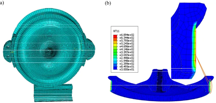
As the material of wheel and rail is the same, the temperature rise in the rail is the same as the temperature drop in case of wheel at a particular instant. Figure 9a shows ABAQUS FE mesh for block-wheel and wheel-rail contacts. This model is developed for the passenger vehicle. Hexagonal and tetrahedral elements are used for meshing the wheel and rail and block, respectively. The wheel, block, brake block holder and rail meshed with 27648, 9641, 6751 and 3918 elements. In this model, heat fluxes qb and qr are given to the blocks and rail, respectively, to estimate temperature field due to braking and contact at the rail. The finite thermal conductance hwr (inverse of thermal contact resistance) at the rail-wheel interface is constant whose value is hwr = 3 × 10⁶ W/m2·°C [31]. It is assumed that heat flux is same for both the blocks (left and right of the wheel) for simplifying the problem. The heat transfer between wheel and rail surface is modeled as qw =qr =hwr(Tw−Tr),
where qw (= qr) are heat flux per unit area, suffices w and r are used for wheel and rail, respectively. The temperature of the rail is assumed to be equal to the ambient temperature (Tr = 30 °C). Since, the contact between wheel and rail and wheel and brake block occurs for a very small span of time, the
thermal penetration depth (
=
a
Pe
) is 6.43 × 10⁻⁵ m (Figure 9b) which is small as compared to thesize of the contact patch.
(a) (b)
Figure 9. (a) Standard 3D FE model of wheel, braking system and rail assembly with meshing and (b)
Temperature distribution on the surface of the wheel.
The influence of the cooling effect of the rail is also implemented here by using convection–diffusion boundary condition. The wheel–block–rail FE model is used to study the heat partitioning between block–wheel and rail–wheel for the above-mentioned brake powers (see Figure
Figure 8.Estimated brake/traction power (Pbrake) (a) at wheel-block and (b) wheel-rail interfaces.
The variation of heat flux on the circumference of the rotating wheel is taken into account while estimating the temperature rise at the tread surface. The generated brake power at the wheel–block interface increases the wheel tread temperature while the wheel and block are in contact and decreases after leaving the braking surface due to convection till the next block is in contact. Again, the temperature of brake block will decrease while the wheel comes in contact with rail due to the rail chill effect.
As the material of wheel and rail is the same, the temperature rise in the rail is the same as the temperature drop in case of wheel at a particular instant. Figure9a shows ABAQUS FE mesh for block-wheel and wheel-rail contacts. This model is developed for the passenger vehicle. Hexagonal and tetrahedral elements are used for meshing the wheel and rail and block, respectively. The wheel, block, brake block holder and rail meshed with 27648, 9641, 6751 and 3918 elements. In this model, heat fluxesqbandqrare given to the blocks and rail, respectively, to estimate temperature field due to braking and contact at the rail. The finite thermal conductancehwr(inverse of thermal contact resistance) at the rail-wheel interface is constant whose value ishwr =3×10⁶W/m2·◦
Vehicles2019,1 97
thermal penetration depth (∆=a/ √
Pe) is 6.43×10⁻⁵m (Figure9b) which is small as compared to the size of the contact patch.
decreases after leaving the braking surface due to convection till the next block is in contact. Again, the temperature of brake block will decrease while the wheel comes in contact with rail due to the rail chill effect.
0 0.5 1 1.5 2 2.5 x10⁶
Pcont
act
(W
att)
Time (s)
400 800 1200
Pbrake
(W
att)
Time (s)
0 400 800 1200
0 5 10 15 x10
7
(a) (b)
0
Figure 8. Estimated brake/traction power (Pbrake) (a) at wheel-block and (b) wheel-rail interfaces.
As the material of wheel and rail is the same, the temperature rise in the rail is the same as the temperature drop in case of wheel at a particular instant. Figure 9a shows ABAQUS FE mesh for block-wheel and wheel-rail contacts. This model is developed for the passenger vehicle. Hexagonal and tetrahedral elements are used for meshing the wheel and rail and block, respectively. The wheel, block, brake block holder and rail meshed with 27648, 9641, 6751 and 3918 elements. In this model, heat fluxes qb and qr are given to the blocks and rail, respectively, to estimate temperature field due to braking and contact at the rail. The finite thermal conductance hwr (inverse of thermal contact resistance) at the rail-wheel interface is constant whose value is hwr = 3 × 10⁶ W/m2·°C [31]. It is assumed that heat flux is same for both the blocks (left and right of the wheel) for simplifying the problem. The heat transfer between wheel and rail surface is modeled as qw =qr =h Twr( w−Tr),
where qw (= qr) are heat flux per unit area, suffices w and r are used for wheel and rail, respectively. The temperature of the rail is assumed to be equal to the ambient temperature (Tr = 30 °C). Since, the contact between wheel and rail and wheel and brake block occurs for a very small span of time, the thermal penetration depth (
Δ =
a
Pe
) is 6.43 × 10⁻⁵ m (Figure 9b) which is small as compared to the size of the contact patch.(a) (b)
Figure 9. (a) Standard 3D FE model of wheel, braking system and rail assembly with meshing and (b) Temperature distribution on the surface of the wheel.
The influence of the cooling effect of the rail is also implemented here by using convection–diffusion boundary condition. The wheel–block–rail FE model is used to study the heat partitioning between block–wheel and rail–wheel for the above-mentioned brake powers (see Figure
Figure 9. (a) Standard 3D FE model of wheel, braking system and rail assembly with meshing and (b) Temperature distribution on the surface of the wheel.
Vehicles2019,1 98
3.4. Material Properties
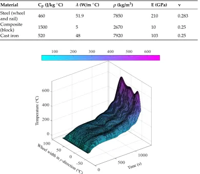
Generally, thermo-mechanical properties of the steel are influenced by temperature variations. In the present research, the temperature dependent mechanical properties of wheel, rail and brake block act as input parameters to the wear model. The wheel and rail are made from steel (pearlite) with composition 0.5 C, 0.7 Mn, 0.3 Si, 0.15 Cr, 0.06 Mo, 0.1 Ni by percentage weight. The brake blocks and brake holders are made of composite material and cast iron, respectively. The physical properties of all the above-mentioned materials are given in Table2. By using all the material properties (Table2) the temperature distribution has been estimated for the total time period (1353 s), which is shown in Figure10.
Table 2.Thermal properties for the wheel and rail, brake blocks and brake holder: Specific heat (Cp), thermal conductivity (λ), mass density (ρ) [2,31].
Material Cp(J/kg◦C) λ(W/m◦C) ρ(kg/m3) E (GPa) ν
Steel (wheel
and rail) 460 51.9 7850 210 0.283
Composite
(block) 1500 5 2670 10 0.25
Cast iron 520 48 7920 103 0.25
Vehicles 2019, 1, FOR PEER REVIEW 11
Table 2. Thermal properties for the wheel and rail, brake blocks and brake holder: Specific heat (Cp),
thermal conductivity (
), mass density (
) [2,31].Material Cp (J/kg °C)
(W/m °C)
(kg/m3) E (GPa) νSteel (wheel and rail) 460 51.9 7,850 210 0.283
Composite (block) 1,500 5 2,670 10 0.25
Cast iron 520 48 7,920 103 0.25
T
em
p
eratu
re
(
oC
)
Figure 10. Temperature distribution on the wheel surface due to tread braking.
4. Wear Evolution Tool
4.1. Contact Model
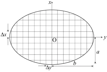
The global contact parameters such as contact forces (longitudinal, lateral and normal), creepage (longitudinal, lateral and spin), rolling radius, contact angle, location of the contact patches and dimensions of the contact patches are collected at each integration step of post-processing of multi-body dynamic simulation in VI-Rail. The local contact parameters such as tangential (lateral and longitudinal) and normal contact pressure and local slip are evaluated within the contact patch from global contact parameters. The normal contact pressure is calculated by the Hertzian contact approach, whereas the tangential pressure and slip are estimated by Kalker’s FASTSIM approach [38], by assuming that the shape of the contact patch is elliptical irrespective of the location of the contact patch. Each contact patch is discretized into cells with ∆y = 2b/(ny − 1) and ∆x(y)= 2a(y)/(nx −
1), where nx and ny are the numbers of cells in x and y directions, respectively as shown in Figure 11.
O
a b
x
y
y x
Figure 11. Discretization of elliptical contact patch.
Figure 10.Temperature distribution on the wheel surface due to tread braking.
Vehicles2019,1 99
4. Wear Evolution Tool 4.1. Contact Model
The global contact parameters such as contact forces (longitudinal, lateral and normal), creepage (longitudinal, lateral and spin), rolling radius, contact angle, location of the contact patches and dimensions of the contact patches are collected at each integration step of post-processing of multi-body dynamic simulation in VI-Rail. The local contact parameters such as tangential (lateral and longitudinal) and normal contact pressure and local slip are evaluated within the contact patch from global contact parameters. The normal contact pressure is calculated by the Hertzian contact approach, whereas the tangential pressure and slip are estimated by Kalker’s FASTSIM approach [38], by assuming that the shape of the contact patch is elliptical irrespective of the location of the contact patch. Each contact patch is discretized into cells with∆y=2b/(ny−1) and∆x(y)=2a(y)/(nx−1), wherenxandnyare the numbers of cells inxandydirections, respectively as shown in Figure11.
Table 2. Thermal properties for the wheel and rail, brake blocks and brake holder: Specific heat (Cp),
thermal conductivity (
λ
), mass density (ρ
) [2,31].Material Cp (J/kg °C)
λ
(W/m °C)ρ
(kg/m3) E (GPa) νSteel (wheel and rail) 460 51.9 7,850 210 0.283
Composite (block) 1,500 5 2,670 10 0.25
Cast iron 520 48 7,920 103 0.25
Te m pe ratu re ( oC)
Figure 10. Temperature distribution on the wheel surface due to tread braking.
4. Wear Evolution Tool
4.1. Contact Model
The global contact parameters such as contact forces (longitudinal, lateral and normal), creepage (longitudinal, lateral and spin), rolling radius, contact angle, location of the contact patches and dimensions of the contact patches are collected at each integration step of post-processing of multi-body dynamic simulation in VI-Rail. The local contact parameters such as tangential (lateral and longitudinal) and normal contact pressure and local slip are evaluated within the contact patch from global contact parameters. The normal contact pressure is calculated by the Hertzian contact approach, whereas the tangential pressure and slip are estimated by Kalker’s FASTSIM approach [38], by assuming that the shape of the contact patch is elliptical irrespective of the location of the contact patch. Each contact patch is discretized into cells with ∆y = 2b/(ny− 1) and ∆x(y) = 2a(y)/(nx− 1), where nx and ny are the numbers of cells in x and y directions, respectively as shown in Figure 11.
O a b x Δ y Δ y x
Figure 11. Discretization of elliptical contact patch. Figure 11.Discretization of elliptical contact patch.
The slip (s) is the combination of rigid slip and the derivative of the relative/elastic displacement between the particles of wheel and rail (u=uw−ur). The slip at any cell (x,y) is calculated as [38]
Vehicles 2019, 1, FOR PEER REVIEW 12
The slip (s) is the combination of rigid slip and the derivative of the relative/elastic displacement between the particles of wheel and rail (u = uw - ur). The slip at any cell (x, y) is
calculated as [38]
( ) (
x y, =υ φ
x− y)
,(
υ φ
y+ y)
T+(
x y t, ,)
s u (9)
where υx,
υ
y andφ
represent longitudinal, lateral and spin creepages [38,39], respectively.In steady-state contact problem, ∂u
( )
x y, ∂ =t 0( )
, ( )( ) (
, ( ),) (
x)
,(
y)
( )x y
x y x y x x y y y y x y
V
υ φ
υ φ
Δ = − − Δ + − + Δ
T
s u u (10)
and the elastic displacement in any grid/mesh within the contact patch is given by
( )
( , )
x y
=
L
tx y
, ,
L L
( , , , , )
ξ
a b G
ν
u
P
=
(11)where L is flexibility function,Pt is the tangential pressure,
ξ
is a global creepage vector, G is shearmodulus and ν is the Poisson’s ratio. The flexibility factor/elasticity coefficient is expressed as
(
)
1 2 sp 3
2 2 2 2
sp ,
x y
x y
L L c L
L c ξ ξ ξ ξ ξ ξ + + =
+ + with L
1 = 8a/ (3Gc11), L2 = 8a/ (3Gc22), L3 =πa a b
(
4c G23)
and c= ab[38,40]. Kalker’s parameter, cij, is a function of a, b and ν. However, the shear modulus depends on
the temperature. The physical properties of the rail and wheel material (both are same) are given in Figure 12. These properties are obtained from several experimentally validated physics-based materials modeling, which are implemented in JMatPro® software [41]. During the experiment to
determine the material parameters, the samples are subjected to the average contact patch pressure which is computed from the contact patch size and the mean axle load. It can be seen that there is significant change in material properties with the temperature. The shear modulus of the material at the contact patch is computed from the elastic modulus and Poisson’s ratio values for the wheel temperature at the given time and location on the track (Figure 10). In Figure 12, the effect of phase transformation is visible as a sudden change in the trend of variation of material with temperature in the temperature range between 600 °C and 800 °C. Thus, the phase transformation effect is implicitly included in the wear evolution model.
0 2000 4000 6000 8000
0 400 800 1200
Temperature (oC)
D en sit y (k g/ m 3) 0 50 100 150 200 250
0 400 800 1200
Temperature(oC)
Y
ou
ng’
s modu
lus(GPa)
Temperature (oC)
Poisson’ s ratio 0 0.15 0.3 0.45 0.6
0 400 800 1200
(a) (b)
(c)
Figure 12. Change in physical properties of the material with temperature: (a) Density, (b) Poisson’s ratio and (c) Young’s modulus or modulus of elasticity.
(9)
whereυx,υyandφrepresent longitudinal, lateral and spin creepages [38,39], respectively. In steady-state contact problem,∂u(x,y)/∂t=0
s(x,y)∆x(y)
V =u(x,y)−u(x−∆x(y),y) + h
(υx−φy),
υy+φy
iT
∆x(y) (10)
and the elastic displacement in any grid/mesh within the contact patch is given by
u(x,y) =LPt(x,y),L=L(ξ,a,b,G,ν) (11) whereLis flexibility function,Ptis the tangential pressure,ξis a global creepage vector,Gis shear modulus andνis the Poisson’s ratio. The flexibility factor/elasticity coefficient is expressed asL=
|ξx|L1+|ξy|L2+c|ξsp|L3
q
(ξ2
x+ξ2y+c2ξ2sp)
, withL1=8a/(3Gc11),L2=8a/(3Gc22),L3=πa √
a/b/(4c23G)andc= √
Vehicles2019,1 100
patch is computed from the elastic modulus and Poisson’s ratio values for the wheel temperature at the given time and location on the track (Figure10). In Figure12, the effect of phase transformation is visible as a sudden change in the trend of variation of material with temperature in the temperature range between 600◦C and 800◦C. Thus, the phase transformation effect is implicitly included in the wear evolution model.
2019, 1, 6 99
The slip (s) is the combination of rigid slip and the derivative of the relative/elastic displacement between the particles of wheel and rail (u = uw - ur). The slip at any cell (x, y) is calculated as [38]
( ) (
x y, =υ φ
x− y)
,(
υ φ
y+ y)
+(
x y t, ,)
T
s u (9)
where υx,
υ
y andφ
represent longitudinal, lateral and spin creepages [38,39], respectively.In steady-state contact problem, ∂u
( )
x y, ∂ =t 0( )
, ( )( ) (
, ( ),) (
x)
,(
y)
( ) x yx y x y x x y y y y x y
V
υ φ
υ φ
Δ = − − Δ + − + Δ
T
s u u (10)
and the elastic displacement in any grid/mesh within the contact patch is given by
( )
( , )
x y
=
L
tx y
, ,
L L
( , , , , )
ξ
a b G
ν
u
P
=
(11)where L is flexibility function,Pt is the tangential pressure,
ξ
is a global creepage vector, G is shearmodulus and ν is the Poisson’s ratio. The flexibility factor/elasticity coefficient is expressed as
(
)
1 2 sp 3
2 2 2 2
sp ,
x y
x y
L L c L
L
c
ξ ξ ξ
ξ ξ ξ
+ +
=
+ + with L1 = 8a/ (3Gc11), L2 = 8a/ (3Gc22), L3=
π
a a b(
4c G23)
and c= ab [38,40]. Kalker’s parameter, cij, is a function of a, b and ν. However, the shear modulus depends on the temperature. The physical properties of the rail and wheel material (both are same) are given in Figure 12. These properties are obtained from several experimentally validated physics-based materials modeling, which are implemented in JMatPro® software [41]. During the experiment to determine the material parameters, the samples are subjected to the average contact patch pressure which is computed from the contact patch size and the mean axle load. It can be seen that there is significant change in material properties with the temperature. The shear modulus of the material at the contact patch is computed from the elastic modulus and Poisson’s ratio values for the wheel temperature at the given time and location on the track (Figure 10). In Figure 12, the effect of phase transformation is visible as a sudden change in the trend of variation of material with temperature in the temperature range between 600 °C and 800 °C. Thus, the phase transformation effect is implicitly included in the wear evolution model.0 2000 4000 6000 8000
0 400 800 1200
Temperature (oC)
D
ensi
ty
(k
g/
m
3)
0 50 100 150 200 250
0 400 800 1200
Temperature(oC)
Y
oung
’s
m
odul
us(GPa)
Temperature (oC)
Poisson’
s ra
tio
0 0.15 0.3 0.45 0.6
0 400 800 1200
(a) (b)
(c)
Figure 12. Change in physical properties of the material with temperature: (a) Density, (b) Poisson’s ratio and (c) Young’s modulus or modulus of elasticity.
Figure 12.Change in physical properties of the material with temperature: (a) Density, (b) Poisson’s ratio and (c) Young’s modulus or modulus of elasticity.
The normal contact pressure for each cell within the elliptical contact patch is estimated in Equation (12) by using Hertz theory. The normal pressure distribution (Pn) [39] at any generic point (x, y), with 1≤x≤nxand 1≤y≤nyis given by
Pn(x,y) =P0 r
1−x 2
a2− y2
b2 (12)
whereP0is the maximum pressure at (0,0).P0= (3N/2πab), whereNstands for normal contact force. If the considered cell inside the contact patch is within the adhesion region (wherePAis the adhesion limit pressure) then
kPA(x,y)k ≤µPn(x,y)⇒Pt(x,y) =PA(x,y), PA(x,y) =Pt(x−∆x(y),y)−
h
(υx−φy),
υy+φy
iT
∆x(y),s(x,y)=0 (13) Otherwise, slip occurs and
kPA(x,y)k> µPn(x,y)⇒
Pt(x,y) =µPn(x,y)PA(x,y)/kPA(x,y)k,
patch, should take place at a higher temperature. However, to simplify the model and computation, such local effects for material parameter variation are not considered in the model developed in this article.
4.2. Wear Model
The wear distribution of the wheel profile is based on the volume of the material removed from the wheel surface, which is related to the total frictional work. Furthermore, due to tread braking, additional heat is generated at the block and the wheel and rail and wheel surfaces due to friction, which is observed in Figure10.
The wear model developed by University of Sheffield (USFD) [42] is used here to estimate wear distribution. This model relates the wear rate, i.e., the weight of the lost material per distance rolled per contact area, to the wear index. Empirical wear constants for three wear regimes, which depend on the contacting materials as well as the frictional power, are introduced. The wear regimes are identified as mild, severe and catastrophic. Tread wear is considered to be in the mild regime whereas flange wear belongs to severe or catastrophic regime. Specific volume (volume per unit area per unit distance travelled (expressed as mm3/mm2m)) is the measure of amount of removal of material at any grid point (x,y), which is a function of time. Wear index (Iwin N/mm2) can be estimated by using the local frictional power developed by tangential contact pressure [40]:
Iw= Pt.s
V (15)
which is based on twin disk experimental data (Figure 13). The data were collected from the experimental test conducted on the roller rig for steel–steel (R8T wheel material and UIC 60 900A rail material) contact bodies under dry condition, presented in [40,43,44]. The wear test results on the twin-disk setup usually have a large spread. Therefore, statistically averaged trends are used to generate the wear map, i.e., the relation between the wear rate and the wear index. The fitted expression for wear rateK(Iw) (inµg/m mm2) is given as
K(Iw) =
5.3Iw, Iw<10.4 N/mm2
55 10.4≤Iw≤77.2 N/mm2
61.9Iw−4723 Iw>77.2 N/mm2
(16)
2019, 1, 6 101
generate the wear map, i.e., the relation between the wear rate and the wear index. The fitted expression for wear rate K (Iw) (in μg/m mm2) is given as
( )
2
w w
2
w w
2
w w
5.3 , 10.4 N / mm 55 10.4 77.2 N/mm 61.9 4723 77.2 N / mm
I I
K I I
I I
<
= ≤ ≤
− >
(16)
Note that the wheel temperature changes the shear modulus G (a function of Young’s modulus and Poisson’s ratio), which in turn changes the flexibility factor L and the elastic displacement u
defined in Equation (11). Therefore, the total slip s defined in Equation (10) becomes dependent on temperature. The local friction power Iw, as defined in Equation (14), depends on the slip s; hence it is influenced by the temperature.
0 500 1000 1500 2000 2500 3000
0 20 40 60 80 100 120
2 w(N/mm ) I
W
ear
ra
te
(μg/m/m
m
2)
K1 K2 K3
Figure 13. Wear map showing the wear rate as a function of wear index [40,43,44].
Generally, the wear rate is different from tread to flange; the wear rate on the tread and flange occur at the regimes K1, and K1 and K2, respectively. The specific volume of the worn material from the wheel can be calculated after evaluating the wear rate as
( )
wp
( )
, K I
x y
δ
ρ
= (17)
The above estimated wear rate (Equation (16)) may be slightly different from the actual wear rate as plastic deformation and fatigue effects are not considered here. Note that the density of the material on the wheel tread changes due temperature (See Figure 12a) and hence the wear rate is doubly influenced by the wheel tread temperatures: first through the dependence of frictional power
w
I on the shear modulus (function of Young’s modulus, Poisson’s ratio and temperature as shown in Figure 12b,c) and, second due to the density
ρ
(in Equation (16)) which also depends on the temperature (Figure 12a). As the temperature increases, there is appreciable reduction in Young’s modulus and a small increase in Poisson’s ratio, which implies that the shear modulus decreases appreciably with increase in temperature. Thus, at increased temperature, the flexibility factors and the frictional power increase. The frictional power determines the regime of wear, and the wear rate K (Iw) (Equation (15)). Further, temperature reduces density. Thus, at higher temperature, the numerator in Equation (16) increases and the denominator decreases. As the material softens due to temperature, more frictional power is generated and the wear rate increases. That is how temperature effects are coupled to the wear rate.The rail–wheel interaction is severely affected by the presence of a third body between their contact, such as wear debris, leaves, wood particles and sand. Usually, soft particulate matter on the rail is instantaneously crushed when the heavily loaded wheel comes over it. Weather conditions such as heat and humidly contributes to rail oxidation and corrosion, and this is especially severe in the coastal areas of India. Oxide formation significantly reduces adhesion/friction under wet condition [45] and similarly, crushed leaf layers reduce friction between the rail and the wheel [45,46]. On one hand, such reduced friction increases the chance of derailment and braking distance
Figure 13.Wear map showing the wear rate as a function of wear index [40,43,44].
Note that the wheel temperature changes the shear modulusG(a function of Young’s modulus and Poisson’s ratio), which in turn changes the flexibility factorL and the elastic displacementu

![Table 1. Parameter values of important components of vehicle [26].](https://thumb-us.123doks.com/thumbv2/123dok_us/9704277.1498072/5.595.88.504.106.421/table-parameter-values-of-important-components-of-vehicle.webp)
![Figure 3.Figure 3. Track between two Indian cities Bhubaneswar and Cuttack at distance 27.9 km [Track between two Indian cities Bhubaneswar and Cuttack at distance 27.9 km [26]](https://thumb-us.123doks.com/thumbv2/123dok_us/9704277.1498072/6.595.98.499.89.257/figure-indian-bhubaneswar-cuttack-distance-bhubaneswar-cuttack-distance.webp)