Simulation of Reinforced Reactive Injection Molding with the Finite Volume Method

(1)

Article

Simulation of Reinforced Reactive Injection Molding

with the Finite Volume Method

Florian Wittemann1,*, Robert Maertens2, Alexander Bernath1ID_{, Martin Hohberg}1_, Luise Kärger1and Frank Henning1,2

1 _{Karlsruhe Institute of Technology (KIT), 76131 Karlsruhe, Germany; [email protected] (A.B.);}

[email protected] (M.H.); [email protected] (L.K.); [email protected] (F.H.) 2 _{Fraunhofer Institute of Chemical Technology (ICT), 76327 Pfinztal, Germany;}

[email protected]

* Correspondence: [email protected]; Tel.: +49-721-60845379

Received: 19 December 2017; Accepted: 22 January 2018; Published: 31 January 2018

Abstract: The reactive process of reinforced thermoset injection molding significantly influences the mechanical properties of the final composite structure. Therefore, reliable process simulation is crucial to predict the process behavior and relevant process effects. Virtual process design is thus highly important for the composite manufacturing industry for creating high quality parts. Although thermoset injection molding shows a more complex flow behavior, state of the art molding simulation software typically focusses on thermoplastic injection molding. To overcome this gap in virtual process prediction, the present work proposes a finite volume (FV) based simulation method, which models the multiphase flow with phase-dependent boundary conditions. Compared to state-of-the-art Finite-Element-based approaches, Finite-Volume-Method (FVM) provides more adequate multiphase flow modeling by calculating the flow at the cell surfaces with an Eulerian approach. The new method also enables the description of a flow region with partial wall contact. Furthermore, fiber orientation, curing and viscosity models are used to simulate the reinforced reactive injection molding process. The open source Computational-Fluid-Dynamics (CFD) toolbox OpenFOAM is used for implementation. The solver is validated with experimental pressure data recorded during mold filling. Additionally, the simulation results are compared to commercial Finite-Element-Method software. The simulation results of the new FV-based CFD method fit well with the experimental data, showing that FVM has a high potential for modeling reinforced reactive injection molding.

Keywords: reinforced reactive injection molding; thermoset processing; process simulation; FVM; OpenFOAM

1. Introduction

Reinforced reactive injection molding (RRIM) is one of the most important manufacturing processes for short fiber reinforced composites with thermoset matrices. The process significantly affects the mechanical and optical properties of the final part. Hence, the process control is crucial for manufacturing high performance parts. Furthermore, an adequate process simulation is needed to achieve this process control and fulfill the high standards of the automotive and polymer industry [1–5].

Despite the importance of the RRIM process, well-known simulation software is often focused on thermoplastic injection molding and uses the same models for RRIM. However, thermosets show a more complex flow behavior, triggered by a low-viscosity surface layer resulting from the hotter mold [1,2,5]. Furthermore, the flow is not shear dominated, like a plug flow, which is a typical adoption for thermoplastics [1,2]. Additionally, commercial software does not simulate the air in the mold as a separate flow phase. This simplification is made to reduce the calculation time, but consequently

(2)

neglects phenomena like air traps with significant influence on the process. These are only taken into account with empirical models in the post processing. For good simulation of RRIM, many material and process aspects need to be considered. As the resin is a non-Newtonian fluid, the viscosity must be modeled as function of temperature, shear rate and degree of cure to accurately simulate the pressure field [6]. For that purpose, and to have a reliable prediction of cycle time, curing kinetics have to be modeled in addition to rate-dependent viscosity models. Furthermore, fiber orientations should be predicted, since they have a significant influence on the mechanical and thermal properties of the final part [3,4,7].

On the one hand, commercial software is often based on the Finite-Element-Method (FEM) to simulate the RRIM process [8–11]. On the other hand, Finite-Volume-based solvers, representing the state of research, focus on thermoplastic injection molding using incompressible and isothermal models [12]. In this study, the Finite-Volume-Method (FVM) is used, resolving the flux at the cell faces and using an Eulerian approach [13–15]. Due to this flow modeling, FVM provides a more realistic multiphase flow with physical significance on the fluxes, which is not possible in FEM by solving a Lagrangian mesh at the nodes. For implementation and simulation, the open source Computational-Fluid-Dynamics (CFD) toolbox OpenFOAM 4.1 (OpenCFD Ltd., Bracknell, UK) [7,12–15] is used and well-known viscosity, curing and fiber orientation models are implemented to model the reinforced reactive injection molding process. A solver for compressible, non-isothermal multiphase flow is extended, using a phase depending boundary condition, defined to enable mold-filling simulation, by separating and interpolating boundary conditions for polymer and air. Additionally, the solver predicts fiber orientation, resulting from the flow during mold filling.

The simulation results are compared to a commercial FEM software (Moldflow 2018.1, Autodesk, San Rafael, CA, USA) and to experimental injection molding trials of a glass fiber reinforced phenolic resin.

2. Models and Implementations

The following subsections present the models and methods used for phase-dependent boundary conditions, curing kinetics, viscosity and fiber orientation. The models are implemented in OpenFOAM 4.1, using C++ as the program language and finite volume theory for the numerical solution [13–15]. In principal, the Navier-Stokes equations can be solved on structured and unstructured meshes. Due to the open source code of the CFD toolbox OpenFOAM, several solvers for scalar transport, transient problems, multiphase problems etc. are available and can be extended in a user-defined way. In the present work, a new solver is created for mold filling simulation of fiber reinforced thermoset materials. The new solver is based on the compressible, non-isothermal multiphase solver compressibleInterFoam. This solver uses the Volume-of–Fluid-Method (VoF) for modeling multiphase flows. VoF separates the different phases using the dimensionless scalarα, which is equal to one in cells completely filled by phase 1, zero in cells filled with phase 2 and 0 <α< 1 in the interface regions [13,15]. In this work,α= 1 means that a control volume is completely filled with polymer resin, andα= 0 if it is filled with air. The boundary conditions of the injection flow are accordingly extended to phase-dependent formulations. Additionally, material models for curing kinetics, viscosity and fiber orientation are implemented to suitably model the reinforced reactive flow behavior.

2.1. Governing Equations

The governing equations are the continuity equation, momentum and energy balance to form the Navier-Stokes equations.

The continuity equation describes the change of the densityρas follows: dρ

dt + ∂(ρUi)

∂xi

(3)

where incompressibility is not assumed, so dρ

dt = 0 is not generally applicable and Ui is the velocity vector.

For momentum balance the general formulation

dρUi dt +

∂ ρUiUj ∂xj

=−∂p

∂xi

+η ∂Ui ∂xj∂xj

(2)

is used withpbeing the pressure andηbeing the viscosity (see Section2.4). The energy balance describes the distribution of the temperatureTwith:

dρT dt +

∂(ρUiT) ∂xi

= λ

cp ∂T ∂xi∂xi

, (3)

according to Fourier’s law. The parametersλ andcp are thermal conductivity and specific heat capacity in this case. The wall temperature of the mold is assumed to be constant, hence no heat transfer between the material and the mold is needed. Radiation is neglected.

2.2. Phase-Dependent Boundary Condition

Three types of boundary faces can be distinguished in OpenFOAM: An inlet for flow into the system, an outlet for flow out of the system and a wall, which cannot be passed by any media. To enable mold-filling simulation, a special boundary condition (BC) for the outlet is developed, which allows the air phase, but not the polymer phase, to leave the mold through the outlet face. Hence, the outlet BC for velocity vectorUis implemented as an interpolation between a Dirichlet boundary condition, defining the absolute value ofUto be zero, and a Neumann boundary condition, defining the gradient ofUto be zero. The interpolation depends on the VoF factorα, in such a way that a cell completely filled with polymer has a pure Dirichlet BC and a cell completely filled with air has a pure Neumann BC. Consequently, the boundary face changes from an outlet to a wall during filling, represented by:

BC=∝·DirichletBC+ (1−α)·NeumannBC, (4)

with

DirichletBC def= U=

  

0 0 0

 

andNeumannBC

def

= dU

dt =   

0 0 0

 

. (5)

For implementation of the phase-dependent BC, a GroovyBC is used, which is part of the third party tool SWAK4FOAM 0.4.1 (Free Software Foundation, Boston, MA, USA). The program code is described in AppendixA.

2.3. Model for Curing Kinetics

Modeling of curing kinetics is an important aspect since cross-linking significantly influences the viscosity and consequently the process pressure and cycle time [16,17]. In this study, the Kamal-Malkin model is used to model curing kinetics, since it is a well-known and often used model for curing kinetics of thermoset polymers [11,16–21]. The model describes the cure rate by

dc

dt = (K1+K2c

m₎₍₁₋_c₎n

(6)

with

K1=A1exp

− E1

R·T

, (7)

K2=A2exp

− E2

R·T

(4)

wherecis the degree of cure between 0 and 1, R is the ideal gas constant andm,n,A1,E1,A2,E2are

material specific constants which have to be identified by experimental measurements like Differential Scanning Calorimetry (DSC) and curve fitting [17]. The curing heat is neglected because of the thin part geometry, hence the curing kinetics have no influence on the temperature distribution. The reaction kinetics model is implemented as a thermo-chemical model within the OpenFOAM structure.

2.4. Model for Viscosity

The Castro-Macosko viscosity model [6] is an often used and well-established model to simulate the viscosity of thermoset materials [11,20,21]. The model describes the viscosity as a function of temperatureT, shear rateγ. and degree of curec:

η T,γ.,c= η0(T) 1+η0(T)

. γ τ∗

(1−n) _c

g cg−c

(c₁+c₂·c)

(9)

and

η0(T) =B·exp

Tb

T

, (10)

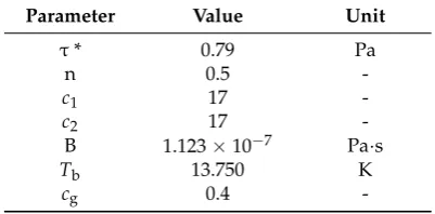
withτ∗,n,c1,c2,BandTbbeing material specific constants. cgdenotes the material specific degree of cure at gelation. The Castro-Macosko model is implemented as a transport model in the thermo-physical model library of OpenFOAM.

2.5. Model for Fiber Orientation

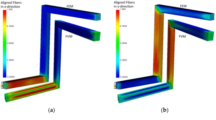
For calculation of the fiber orientations, the Folgar Tucker model is used [22–25]. A well-described implementation of this model has already been published by Kerstin Heinen [7]. Heinen’s code is extended in the present work to model multiphase flows. Hence, fiber orientation is calculated only in cells withα≥0.5. In all other cells the initial conditions remain. The result is a symmetric tensor [23], with the diagonal entries being the probability of fibers oriented in this coordinate direction with a value between zero and one, where zero means no fibers are aligned in this direction and one, that all fibers are aligned in this direction. The summation of the diagonal entries must be equal to one.

The fourth order fiber orientation tensorAklij is described by second order tensors using the hybrid closure approximation, as described in [7,23,24]. The differential equation for the second order fiber orientation tensor in a control volume is given by:

dAij dt +

∂viAjk ∂xk

=−WikAkj−AikWkj

+λF

DikAkj−AikDkj−2DklAklij

+2CI

.

γ δij−3Aij

, (11)

with

Dij= 1 2

∂Ui ∂xj

+1

2 ∂Ui ∂xj

!T

(12)

Wij = 1 2

∂Ui ∂xj

−1 2

∂Ui ∂xj

!T

(13)

λF = r

2₋₁

r2₊₁ (14)

(5)

3. Test Setup for Experimental Validation

3.1. Test Structure and Process Conditions

The thermoset molding compound used for the experimental studies is a phenolic resin of the novolac type, reinforced with glass fibers. The material was provided for the trials by SBHPP Vyncolit (Gent, Belgium).

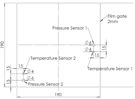
For the experimental study, an electrically heated plate mold equipped with pressure and temperature sensors is used. It is a symmetrical two-cavity mold with a variable plate thickness between two and five millimeters. For the experimental studies described here, a constant wall thickness of 2 mm is chosen. Both plates have a square shape with an edge length of 190 mm. The sprue has a start diameter of 9 mm (inlet), expands to 15.5 mm and is 185 mm high. Figure1 shows the complete molded part with sprue system. The position of the pressure and temperature sensors in one of the mold cavities is shown in Figure2.

J. Compos. Sci. 2017, 1, x FOR PEER REVIEW 5 of 16

For the experimental study, an electrically heated plate mold equipped with pressure and temperature sensors is used. It is a symmetrical two-cavity mold with a variable plate thickness between two and five millimeters. For the experimental studies described here, a constant wall thickness of 2 mm is chosen. Both plates have a square shape with an edge length of 190 mm. The sprue has a start diameter of 9 mm (inlet), expands to 15.5 mm and is 185 mm high. Figure 1 shows the complete molded part with sprue system. The position of the pressure and temperature sensors in one of the mold cavities is shown in Figure 2.

Figure 1. Molded part with sprue system.

Figure 2. Position of pressure and temperature sensors in mold.

The sensor positions are in the region where the first material should appear after entering the plate mold (position 1) and the last region where material should appear before complete filling (position 2). The positions are chosen to see when the plate filling starts and ends. The sensors are nearly in plane with the mold, so the influence on material flow behavior can be neglected. For pressure measurement, sensors of the type 6163 manufactured by Kistler Instrumente GmbH (Winterhur, Switzerland) are used. These sensors are equipped with a diaphragm in order to resist the low viscosity resin. The temperature sensors are Kistler type 6192 NiCr-Ni thermocouples. The injection molding machine is a KraussMaffei 550/2000 GX (Munich, Germany) equipped with a standard 60 mm thermoset screw without a non-return valve. The temperature control of the plasticizing unit is realized using four individually controlled, oil-tempered zones. The clamping unit has a maximum clamping force of 5500 kN.

Figure 1.Molded part with sprue system.

For the experimental study, an electrically heated plate mold equipped with pressure and temperature sensors is used. It is a symmetrical two-cavity mold with a variable plate thickness between two and five millimeters. For the experimental studies described here, a constant wall thickness of 2 mm is chosen. Both plates have a square shape with an edge length of 190 mm. The sprue has a start diameter of 9 mm (inlet), expands to 15.5 mm and is 185 mm high. Figure 1 shows the complete molded part with sprue system. The position of the pressure and temperature sensors in one of the mold cavities is shown in Figure 2.

Figure 1. Molded part with sprue system.

Figure 2. Position of pressure and temperature sensors in mold.

The sensor positions are in the region where the first material should appear after entering the plate mold (position 1) and the last region where material should appear before complete filling (position 2). The positions are chosen to see when the plate filling starts and ends. The sensors are nearly in plane with the mold, so the influence on material flow behavior can be neglected. For pressure measurement, sensors of the type 6163 manufactured by Kistler Instrumente GmbH (Winterhur, Switzerland) are used. These sensors are equipped with a diaphragm in order to resist the low viscosity resin. The temperature sensors are Kistler type 6192 NiCr-Ni thermocouples. The injection molding machine is a KraussMaffei 550/2000 GX (Munich, Germany) equipped with a standard 60 mm thermoset screw without a non-return valve. The temperature control of the plasticizing unit is realized using four individually controlled, oil-tempered zones. The clamping unit has a maximum clamping force of 5500 kN.

Figure 2.Position of pressure and temperature sensors in mold.

(6)

The injection molding machine is a KraussMaffei 550/2000 GX (Munich, Germany) equipped with a standard 60 mm thermoset screw without a non-return valve. The temperature control of the plasticizing unit is realized using four individually controlled, oil-tempered zones. The clamping unit has a maximum clamping force of 5500 kN.

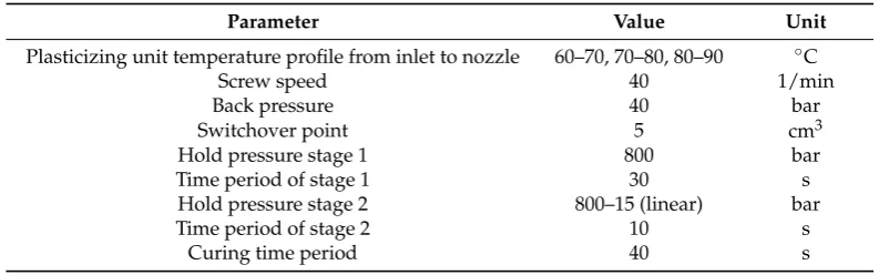
The process parameters for obtaining the pressure and temperature signals are summarized in Tables1and2.

Table 1.Constant process parameters used in the RRIM study.

Parameter Value Unit

Plasticizing unit temperature profile from inlet to nozzle 60–70, 70–80, 80–90 ◦C

Screw speed 40 1/min

Back pressure 40 bar

Switchover point 5 cm3

Hold pressure stage 1 800 bar

Time period of stage 1 30 s

Hold pressure stage 2 800–15 (linear) bar

Time period of stage 2 10 s

Curing time period 40 s

Table 2.Varied parameters used in the RRIM study.

Parameter Value Min Value Max Unit

Mold temperature 170 190 ◦C

Injection speed 137.5 250 cm3/s

Dosage volume 230 232 cm3

The filling is injection speed controlled until the switchover point, meaning that there is a constant material inflow until 5 cm3of the dosage volume remains in the plasticizing unit. After the switchover, a constant pressure (hold pressure) acts on the inlet. After the hold pressure stages, the mold is separated from the plasticizing unit and no material flow in the mold is possible. The curing time ensures the shape stability of the composite part.

The aim of this study is to investigate the flow behavior with dependence on varying mold temperature and injection speed and, thus, to validate the proposed FVM-based CFD method. In order to compensate the difference in material backflow at higher injection speeds, the dosage volume is adapted accordingly. The purpose of this adaption is to keep the maximum cavity pressure constant within the study.

3.2. Numerical Model, Boundary Conditions and Model Parameters

Since the mold is symmetric in two directions (cf. Figure1), only a quarter of the mold is simulated to reduce the computation time. The model with predefined boundary face types is shown in Figure3. To replicate the experiments, four simulations with different process settings are conducted. Thus, two different injection speeds and two different mold temperatures are modeled. For pressure validation, the FVM-based solver is compared to the experimental results and also to FEM results. The FEM simulations are conducted with Autodesk Moldflow Insight 2018.1, also using Castro-Macosko viscosity and the Kamal-Malkin kinetic model [8–10]. The FEM model is meshed in Moldflow with a global edge length of 3.06 mm and eight elements over thickness. The FVM model is meshed with the OpenFOAM meshing tools BlockMesh and snappyHexMesh. Therefore, a base mesh with an edge length 2 mm is used, the refinement of all surfaces is set to level 2 and one additional surface layer is created.

(7)

The hydrostatic pressure is given by the scalarprgh. In this study it is equal to the pressurep,

because gravity is neglected.

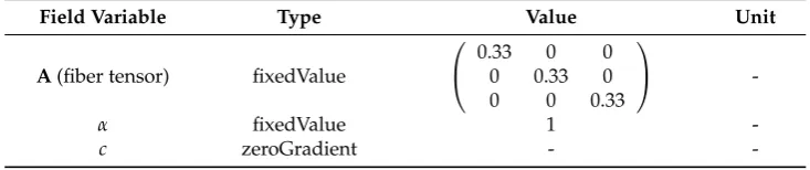
At the symmetry planes the symmetry condition is set for every field variable. The flow rate at the inlet in Table4equals one quarter of 137.5 cm3/s and 250 cm3/s, because only one quarter of the mold is simulated. According to the experiments, the filling simulation is initially volume-flux controlled (Table4), and pressure-controlled after the first switchover point. Two switchover points are also used in the FEM and FVM simulations, where the FVM settings are chosen according to the FEM simulations: After the first switchover point, the pressure is set constant at the actual values, calculated for this time step. After the second one, the pressure is set according to the holding pressure of the experiments, see Table1. At the first switchover point, the inlet boundary condition for the velocity is changed to pressureInletOutletVelocity, so that the velocity is calculated relating to the fixed pressure. The switchover points are calculated from the experimental parameters and the mold volume. They are given in Table7.

are also used in the FEM and FVM simulations, where the FVM settings are chosen according to the FEM simulations: After the first switchover point, the pressure is set constant at the actual values, calculated for this time step. After the second one, the pressure is set according to the holding pressure of the experiments, see Table 1. At the first switchover point, the inlet boundary condition for the velocity is changed to pressureInletOutletVelocity, so that the velocity is calculated relating to the fixed pressure. The switchover points are calculated from the experimental parameters and the mold volume. They are given in Table 7.

Figure 3. Finite-Volume-Method (FVM) model for OpenFOAM with boundary faces.

Table 3. Initial conditions and values for the internal field.

Field Variable Value Unit

A (fiber tensor)

0.33 0 0 0 0.33 0

0 0 0.33 -

α 0 -

c 0.001 -

cure rate 0 1/s

0 1/s

p and prgh 105 Pa

T 443.15 or 463.15 K

U (0 0 0) m/s

Table 4. Boundary conditions and values for the inlet.

Field Variable Type Value Unit

A (fiber tensor) fixedValue

0.33 0 0 0 0.33 0

0 0 0.33 -

α fixedValue 1 -

c zeroGradient - -

cure rate zeroGradient - 1/s

zeroGradient - 1/s

p and prgh fixedfluxPressure 105 Pa

T fixedValue 423.15 K

U flowRateInletVelocity 34.375 × 10−6 _{or 62.5}_∙_{× 10}−6 _m3_/s

Figure 3.Finite-Volume-Method (FVM) model for OpenFOAM with boundary faces.

Table 3.Initial conditions and values for the internal field.

Field Variable Value Unit

A(fiber tensor) 



0.33 0 0

0 0.33 0

0 0 0.33





-α 0

-c 0.001

-cure rate 0 1/s

.

γ 0 1/s

pandp_rgh 105 _Pa

T 443.15 or 463.15 K

U (0 0 0) m/s

Table 4.Boundary conditions and values for the inlet.

A(fiber tensor) fixedValue





0.33 0 0

0 0.33 0

0 0 0.33





-α fixedValue 1

(8)

-Table 4.Cont.

cure rate zeroGradient - 1/s

.

γ zeroGradient - 1/s

pandprgh fixedfluxPressure 105 Pa

T fixedValue 423.15 K

U flowRateInletVelocity 34.375×10−6or 62.5×10−6 m3/s

Table 5.Boundary conditions and values for the outlet.

A(fiber tensor) zeroGradient -

-α zeroGradient -

-cure zeroGradient -

-cure rate zeroGradient - 1/s

gammadot zeroGradient - 1/s

pandprgh zeroGradient - Pa

T fixedValue 443.15 or 463.15 K

U BC (see Section2.2) - m/s

Table 6.Boundary conditions and values for the wall.

A(fiber tensor) zeroGradient -

-α zeroGradient -

-cure zeroGradient -

-cureRate zeroGradient - 1/s

gammadot zeroGradient - 1/s

pandprgh fixedfluxPressure 105 Pa

T fixedValue 443.15 or 463.15 K

U noSlip - m/s

For fiber orientation prediction, a fiber volume fraction of 0.35 and an aspect ratio of 25 are assumed.

Table 7.Switchover points of the simulations.

Filling Rate First Point Second Point

137.5 cm3/s 1.46 s 1.5 s

250 cm3/s 0.8 s 0.82 s

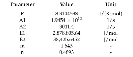
Table8summarizes the parameter values of reaction kinetics of the material system used for experimental validation.

Table 8.Parameters for the Kamal-Malkin kinetic model.

R 8.3144598 J/(K·mol)

A1 1.9454×1012 _1/s

A2 3041.4 1/s

E1 2,878,805.64 J/mol

E2 38,425.6452 J/mol

m 1.643

(9)

-The parameter values of the viscosity model of the material system used for experimental validation are given in Table9. Air is assumed to be a perfect gas.

Table 9.Parameters for the Castro-Macosko viscosity model.

τ* 0.79 Pa

n 0.5

-c1 17

-c2 17

-B 1.123×10−7 Pa·s

Tb 13.750 K

cg 0.4

-Values received from manufacturer.

3.3. Numerical Model for Verification of Fiber Orientations

For comparison of fiber orientation results of FVM and FEM a different geometry is regarded. To verify all room directions, a mold with dominant flow in every direction is created. The boundary types are the same as mentioned in Tables5–8. Geometry and boundary faces are shown in Figure4. For the velocity, an injection speed of 3.8 cm3/s is chosen, leading to a filling time of 1 s. The inlet and outlet are squares with an edge length of 5 mm. The FEM mesh is built up in Moldflow with tetrahedral elements, while hexahedral volumes created with BlockMesh are used for the FVM mesh. In both meshes a global edge length of 1 mm is set.

Table 9. Parameters for the Castro-Macosko viscosity model.

Parameter Value Unit

τ* 0.79 Pa

n 0.5 - 17 - 17 -

B 1.123∙× 10−7_Pa_∙_s

Tb 13.750 K

cg 0.4

-* Values received from manufacturer.

3.3. Numerical Model for Verification of Fiber Orientations

For comparison of fiber orientation results of FVM and FEM a different geometry is regarded. To verify all room directions, a mold with dominant flow in every direction is created. The boundary types are the same as mentioned in Tables 5–8. Geometry and boundary faces are shown in Figure 4. For the velocity, an injection speed of 3.8 cm3_{/s is chosen, leading to a filling time of 1 s. The inlet}

and outlet are squares with an edge length of 5 mm. The FEM mesh is built up in Moldflow with tetrahedral elements, while hexahedral volumes created with BlockMesh are used for the FVM mesh. In both meshes a global edge length of 1 mm is set.

Figure 4. Geometry for fiber orientation validation.

4. Results

In this section, the simulation results are presented and compared to experimental and FEM results.

4.1. Results of the Filling Simulation

Figure 5 shows the FVM simulation results for a filling rate of 137.5 cm3_{/s and a mold temperature of}

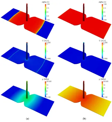
170 °C. Displayed are (from top to bottom) the filling level (via VoF), the velocity in m/s and the pressure in MPa at 1 s (Figure 5a), where the filling is velocity-controlled, and at 1.5 s (Figure 5b), where it is pressure-controlled and should be just filled.

At 1.5 s the mold is not filled completely, visible at the corners, where air is still left in the system (blue). For a sum of α over all cells, divided by the total number of cells, the value should be equal to one for a complete filled system. In this case, the value is 0.998, which matches a filling state of 99.8%. The 0.2% air can be neglected and the mold is regarded as completely filled. The mold gets completely

Figure 4.Geometry for fiber orientation validation.

4. Results

In this section, the simulation results are presented and compared to experimental and FEM results.

4.1. Results of the Filling Simulation

(10)

At 1.5 s the mold is not filled completely, visible at the corners, where air is still left in the system (blue). For a sum ofαover all cells, divided by the total number of cells, the value should be equal to one for a complete filled system. In this case, the value is 0.998, which matches a filling state of 99.8%. The 0.2% air can be neglected and the mold is regarded as completely filled. The mold gets completely filled during holding pressure stage 1. There is no possibility to make a statement when exactly the mold in the trials is filled completely, because the material can only be detected at the sensor points. Based on the pressure data, the pressure rise and difference between sensor 1 and 2 in the trials, the filling also takes approximately 1.5 s for an injection speed of 137.5 cm3/s in the experimental studies (see Section4.2).

A detailed look at the flow front (Figure5a top) displays that there is no sharp interface between polymer and air, but an interface region with 0 <α≤1 over a few cells. This area indicates the region with partial wall contact, which is a typical phenomenon of RRIM, although a clear line between partial and full wall contact is not detectable as described in [1,2,5]. This phenomenon cannot be observed in the FEM simulation, where a sharp interface is predicted and an element is always either polymer or empty, see Figure6.

filled during holding pressure stage 1. There is no possibility to make a statement when exactly the mold in the trials is filled completely, because the material can only be detected at the sensor points. Based on the pressure data, the pressure rise and difference between sensor 1 and 2 in the trials, the filling also takes approximately 1.5 s for an injection speed of 137.5 cm3_{/s in the experimental studies} (see Section 4.2).

A detailed look at the flow front (Figure 5a top) displays that there is no sharp interface between polymer and air, but an interface region with 0 < α≤ 1 over a few cells. This area indicates the region with partial wall contact, which is a typical phenomenon of RRIM, although a clear line between partial and full wall contact is not detectable as described in [1,2,5]. This phenomenon cannot be observed in the FEM simulation, where a sharp interface is predicted and an element is always either polymer or empty, see Figure 6.

(a) (b)

Figure 5. FVM-simulation results of polymer filling state alpha (top), velocity U in m/s (middle) and pressure p in MPa (bottom) after 1 s (a) and 1.5 s (b) for a filling rate of 137.5 cm3_{/s and a mold} temperature of 170 °C.

(11)

J. Compos. Sci. 2018,2, 5 11 of 16

Figure 6. Filling state of the FEM-simulation at 1 s.

The velocity (Figure 5 middle) ranges in a reasonable spectrum. The polymer enters the mold with an injection speed of 2.2 m/s at the inlet, which corresponds to a volumetric flow rate of 137.5 cm3/s based on the inlet area. Furthermore, it can be seen that the velocity is nearly zero after 1.5 s (Figure 5b middle), although there is still a pressure gradient at that moment (Figure 5 bottom). This aspect approves the phase-dependent boundary condition, which stops the flow when the mold is filled.

4.2. Comparisson of Pressure

The pressure during filling with an injection speed of 137.5 cm3_{/s is shown in Figure 7a for a}

mold temperature of 170 °C and Figure 7b for 190 °C. The experiments at 170 °C are more reproducible than the ones at 190 °C, as visualized by the scatter beams in Figure 7. The large scatter at 190 °C might be caused by the fact that 190 °C is the maximum temperature for injection molding according to the manufacturer. Every curve of sensor position 1 shows a continuous pressure growth during filling (0–1.46 s). After filling, the experimental curves of sensor 1 and 2 are nearly identical, which shows good process control and filling behavior. The simulation results of FEM and FVM considerably differ from each other. Compared to measurements at sensor 1, FEM predicts a higher pressure, while the FVM results fit better to the experiments and are just slightly higher for 170 °C. At sensor 2, a significant pressure rise after switchover (1.46 s) is detectable in experiments as well as in FEM and FVM simulations. However, both simulations show a too fast pressure rise at sensor 2 compared to the measurements.

0.0 0.5 1.0 1.5 2.0

0 5 10 15 20 25 Measurement FEM_singlephase FVM_multiphase Sensor1 Sensor2 Pr essu re [MPa ] Time [s]

0.0 0.5 1.0 1.5 2.0

0 5 10 15 20 25 Measurement FEM_singlephase FVM_multiphase Sensor1 Sensor2 Pr es su re [M Pa ] Time [s] (a) (b)

Figure 7. Pressure over time for a filling speed of 137.5 cm3_{/s and a mold temperature of 170 °C (}_a₎ and 190 °C (b). Comparing measurement (black), FEM (red) and FVM (blue) at sensor position 1 (solid line) and 2 (dotted line).

Figure 6.Filling state of the FEM-simulation at 1 s.

The velocity (Figure5middle) ranges in a reasonable spectrum. The polymer enters the mold with an injection speed of 2.2 m/s at the inlet, which corresponds to a volumetric flow rate of 137.5 cm3/s based on the inlet area. Furthermore, it can be seen that the velocity is nearly zero after 1.5 s (Figure5b middle), although there is still a pressure gradient at that moment (Figure5bottom). This aspect approves the phase-dependent boundary condition, which stops the flow when the mold is filled.

4.2. Comparisson of Pressure

The pressure during filling with an injection speed of 137.5 cm3/s is shown in Figure7a for a mold temperature of 170◦C and Figure7b for 190◦C. The experiments at 170◦C are more reproducible than the ones at 190◦C, as visualized by the scatter beams in Figure7. The large scatter at 190◦C might be caused by the fact that 190◦C is the maximum temperature for injection molding according to the manufacturer. Every curve of sensor position 1 shows a continuous pressure growth during filling (0–1.46 s). After filling, the experimental curves of sensor 1 and 2 are nearly identical, which shows good process control and filling behavior. The simulation results of FEM and FVM considerably differ from each other. Compared to measurements at sensor 1, FEM predicts a higher pressure, while the FVM results fit better to the experiments and are just slightly higher for 170◦C. At sensor 2, a significant pressure rise after switchover (1.46 s) is detectable in experiments as well as in FEM and FVM simulations. However, both simulations show a too fast pressure rise at sensor 2 compared to the measurements.

Figure 6. Filling state of the FEM-simulation at 1 s.

The velocity (Figure 5 middle) ranges in a reasonable spectrum. The polymer enters the mold with an injection speed of 2.2 m/s at the inlet, which corresponds to a volumetric flow rate of 137.5 cm3/s based on the inlet area. Furthermore, it can be seen that the velocity is nearly zero after 1.5 s (Figure 5b middle), although there is still a pressure gradient at that moment (Figure 5 bottom). This aspect approves the phase-dependent boundary condition, which stops the flow when the mold is filled.

4.2. Comparisson of Pressure

The pressure during filling with an injection speed of 137.5 cm3_{/s is shown in Figure 7a for a}

mold temperature of 170 °C and Figure 7b for 190 °C. The experiments at 170 °C are more reproducible than the ones at 190 °C, as visualized by the scatter beams in Figure 7. The large scatter at 190 °C might be caused by the fact that 190 °C is the maximum temperature for injection molding according to the manufacturer. Every curve of sensor position 1 shows a continuous pressure growth during filling (0–1.46 s). After filling, the experimental curves of sensor 1 and 2 are nearly identical, which shows good process control and filling behavior. The simulation results of FEM and FVM considerably differ from each other. Compared to measurements at sensor 1, FEM predicts a higher pressure, while the FVM results fit better to the experiments and are just slightly higher for 170 °C. At sensor 2, a significant pressure rise after switchover (1.46 s) is detectable in experiments as well as in FEM and FVM simulations. However, both simulations show a too fast pressure rise at sensor 2 compared to the measurements.

0.0 0.5 1.0 1.5 2.0

0 5 10 15 20 25 Measurement FEM_singlephase FVM_multiphase Sensor1 Sensor2 Pr essu re [MPa ] Time [s]

0.0 0.5 1.0 1.5 2.0

0 5 10 15 20 25 Measurement FEM_singlephase FVM_multiphase Sensor1 Sensor2 Pr es su re [M Pa ] Time [s] (a) (b)

Figure 7. Pressure over time for a filling speed of 137.5 cm3_{/s and a mold temperature of 170 °C (}_a₎ and 190 °C (b). Comparing measurement (black), FEM (red) and FVM (blue) at sensor position 1 (solid line) and 2 (dotted line).

(12)

The pressure difference between sensor 1 and 2 after switchover is too high in both simulations for both temperatures, where it is even higher in the FEM than in the FVM calculations. In general, the pressure during filling is lower at 190◦C than for 170◦C in experiments and simulations. This is caused by the lower viscosity, resulting from the higher temperature.

Although material backflow is not simulated, the overall pressure rise at both sensor positions is quite similar in experiments and simulations. Hence, material backflow could be neglected, although no non-return valve is used in the experimental trials.

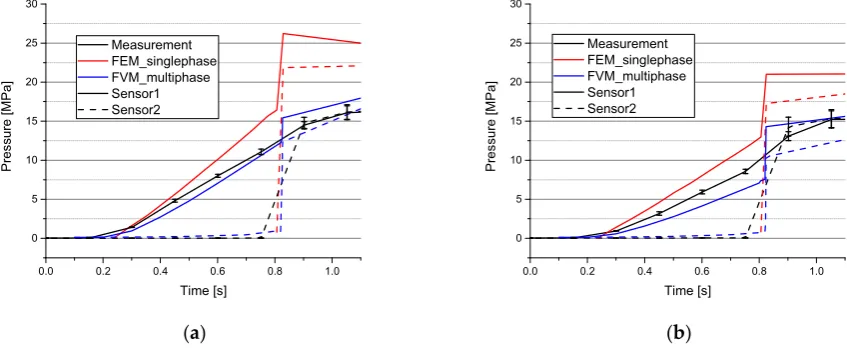
For a filling rate of 250 cm3/s, there is also a greater scatter in pressure measurement for 190◦C (Figure8b) than for 170◦C (Figure8a) and the pressure is again lower at 190◦C because of the lower viscosity. Up to the first switchover, the experimental data of a filling rate of 250 cm3_{/s show a higher}

pressure growth during filling than the data of the filling rate of 137.5 cm3/s (Figure7), which is a consequence of the higher velocity. Hence, there is no visible pressure rise at switchover (0.8 s) for sensor 1. After switchover, the experimental curves of sensor 1 and 2 do not immediately fit to each other as well as for 137.5 cm3/s. For 190◦C the measured pressure at sensor 2 is even higher than the one at sensor 1 between 0.85 and 1 s.

The pressure difference between sensor 1 and 2 after switchover is too high in both simulations for both temperatures, where it is even higher in the FEM than in the FVM calculations. In general, the pressure during filling is lower at 190 °C than for 170 °C in experiments and simulations. This is caused by the lower viscosity, resulting from the higher temperature.

Although material backflow is not simulated, the overall pressure rise at both sensor positions is quite similar in experiments and simulations. Hence, material backflow could be neglected, although no non-return valve is used in the experimental trials.

For a filling rate of 250 cm3_{/s, there is also a greater scatter in pressure measurement for 190 °C}

(Figure 8b) than for 170 °C (Figure 8a) and the pressure is again lower at 190 °C because of the lower viscosity. Up to the first switchover, the experimental data of a filling rate of 250 cm3_{/s show a higher}

pressure growth during filling than the data of the filling rate of 137.5 cm3_{/s (Figure 7), which is a}

consequence of the higher velocity. Hence, there is no visible pressure rise at switchover (0.8 s) for sensor 1. After switchover, the experimental curves of sensor 1 and 2 do not immediately fit to each other as well as for 137.5 cm3_{/s. For 190 °C the measured pressure at sensor 2 is even higher than the}

one at sensor 1 between 0.85 and 1 s.

0.0 0.2 0.4 0.6 0.8 1.0

0 5 10 15 20 25 30 Measurement FEM_singlephase FVM_multiphase Sensor1 Sensor2 P res sure [MPa] Time [s]

0.0 0.2 0.4 0.6 0.8 1.0

0 5 10 15 20 25 30 Measurement FEM_singlephase FVM_multiphase Sensor1 Sensor2 P res sure [MPa] Time [s] (a) (b)

Figure 8. Pressure as a function of time for a filling speed of 250 cm3_{/s and a mold temperature of 170 °C} (a) and 190 °C (b). Comparing measurement (black), FEM (red) and FVM (blue) at sensor Position 1 (solid line) and 2 (dotted line).

Both simulation methods overestimate the pressure rise at switchover, which is distinctly higher in the FEM simulations. As before, the FEM calculated pressure is too high for sensor 1. The pressure distribution of the FVM simulation fits well during filling for 170 °C and is too low for 190 °C. Regarding the curve course of sensor 2, the pressure rise of both methods appears too fast. However, the real pressure curve in this area is not entirely known, because there are only measure points at 0.75 and 0.9 s (switchover at 0.8 s), making the distribution look flatter.

In summary, the results of the FVM simulation are satisfying, although no further material characterization has been done except for the material data provided by the manufacturer. By ranging in a correct spectrum and rising at the right time, the FVM simulation results show a good agreement with the experimental data. The proper pressure modeling indicates a suitable viscosity modeling and hence a suitable simulation of curing kinetics, as further evaluated in the following section.

4.3. Comparison of Curing Kinetics

The correct implementation of the curing kinetics modeling of the new FVM-solver is verified by comparison with commercial FEM software, which also uses the Kamal-Malkin model. The increase of the curing degree at sensor position 1 is illustrated in Figure 9. The results are quite similar for FEM and FVM, confirming the correct implementation in the curing kinetics modeling in the FVM-solver. At the end of filling (1.5 s) the degree of cure is about 0.85% (in the FVM simulation).

Figure 8.Pressure as a function of time for a filling speed of 250 cm3/s and a mold temperature of 170 ◦C (a) and 190◦C (b). Comparing measurement (black), FEM (red) and FVM (blue) at sensor Position 1 (solid line) and 2 (dotted line).

Both simulation methods overestimate the pressure rise at switchover, which is distinctly higher in the FEM simulations. As before, the FEM calculated pressure is too high for sensor 1. The pressure distribution of the FVM simulation fits well during filling for 170 ◦C and is too low for 190◦C. Regarding the curve course of sensor 2, the pressure rise of both methods appears too fast. However, the real pressure curve in this area is not entirely known, because there are only measure points at 0.75 and 0.9 s (switchover at 0.8 s), making the distribution look flatter.

In summary, the results of the FVM simulation are satisfying, although no further material characterization has been done except for the material data provided by the manufacturer. By ranging in a correct spectrum and rising at the right time, the FVM simulation results show a good agreement with the experimental data. The proper pressure modeling indicates a suitable viscosity modeling and hence a suitable simulation of curing kinetics, as further evaluated in the following section.

4.3. Comparison of Curing Kinetics

(13)

At the end of filling (1.5 s) the degree of cure is about 0.85% (in the FVM simulation). This raises the viscosity by 44.5% (Equation (9)) related to the same temperature and shear rate but with a degree of curing equal to zero (c= 0).

The kinetic model (see Section2.3) only depends on the state variables time and temperature, which are not as much influenced by flow as pressure and velocity. That might be the reason for the good fitting results of FEM and FVM.

This raises the viscosity by 44.5% (Equation (9)) related to the same temperature and shear rate but with a degree of curing equal to zero (c = 0).

The kinetic model (see Section 2.3) only depends on the state variables time and temperature, which are not as much influenced by flow as pressure and velocity. That might be the reason for the good fitting results of FEM and FVM.

0 20 40 60 80

0.0 0.2 0.4 0.6 0.8 1.0

De

gree

of

C

ur

e [

-]

Time [s] FEM

FVM

Figure 9. Degree of cure as a function of time for FEM (black) and FVM (red) for a filling speed of 137.5 cm3_{/s and a mold temperature of 170 °C.}

4.4. Comparison of Fiber Orientation

The fiber orientation computed by FVM simulation is compared to those of commercial FEM software. For the FEM simulation, the Moldflow standard model (Moldflow-rotation-diffusion) is chosen. The results are based on the geometry of Figure 4. The geometries in Figure 10 might seem to be different for FEM and FVM, which is only caused by the perspective.

Regarding the fiber alignment in x-direction (Figure 10a), a deviation especially in the edges can be detected. In the FEM model, a high orientation right at the beginning can be detected, while the FVM result aligns only after a few millimeters. The results in y-direction fit well, while in z-direction the FVM-solver predicts a slightly higher alignment of about 10%. The FVM solution has a higher scattering in the transition area.

(a) (b)

Figure 9.Degree of cure as a function of time for FEM (black) and FVM (red) for a filling speed of 137.5 cm3/s and a mold temperature of 170◦C.

4.4. Comparison of Fiber Orientation

The fiber orientation computed by FVM simulation is compared to those of commercial FEM software. For the FEM simulation, the Moldflow standard model (Moldflow-rotation-diffusion) is chosen. The results are based on the geometry of Figure4. The geometries in Figure10might seem to be different for FEM and FVM, which is only caused by the perspective.

Regarding the fiber alignment inx-direction (Figure10a), a deviation especially in the edges can be detected. In the FEM model, a high orientation right at the beginning can be detected, while the FVM result aligns only after a few millimeters. The results iny-direction fit well, while inz-direction the FVM-solver predicts a slightly higher alignment of about 10%. The FVM solution has a higher scattering in the transition area.

This raises the viscosity by 44.5% (Equation (9)) related to the same temperature and shear rate but with a degree of curing equal to zero (c = 0).

The kinetic model (see Section 2.3) only depends on the state variables time and temperature, which are not as much influenced by flow as pressure and velocity. That might be the reason for the good fitting results of FEM and FVM.

0 20 40 60 80

0.0 0.2 0.4 0.6 0.8 1.0

De

gree

of

C

ur

e [

-]

Time [s] FEM

FVM

Figure 9. Degree of cure as a function of time for FEM (black) and FVM (red) for a filling speed of 137.5 cm3_{/s and a mold temperature of 170 °C.}

4.4. Comparison of Fiber Orientation

The fiber orientation computed by FVM simulation is compared to those of commercial FEM software. For the FEM simulation, the Moldflow standard model (Moldflow-rotation-diffusion) is chosen. The results are based on the geometry of Figure 4. The geometries in Figure 10 might seem to be different for FEM and FVM, which is only caused by the perspective.

Regarding the fiber alignment in x-direction (Figure 10a), a deviation especially in the edges can be detected. In the FEM model, a high orientation right at the beginning can be detected, while the FVM result aligns only after a few millimeters. The results in y-direction fit well, while in z-direction the FVM-solver predicts a slightly higher alignment of about 10%. The FVM solution has a higher scattering in the transition area.

(a) (b)

(14)

(c)

Figure 10. Comparison of predicted fiber orientation between FEM and FVM in x-direction (a), y -direction (b) and z-direction (c).

These slight differences may be caused by the different flow modeling. The plug flow, modeled in FEM, allows a faster orientation especially in regions near the walls (like edges and corners) because of the full wall contact, whereas the fountain flow with partial wall contact modeled in FVM does not lead to such a rapid orientation, because of the different velocity gradient. In summary the results fit well, which confirms a correct implementation.

5. Discussion and Conclusions

A new method for simulation of reinforced reactive injection molding is presented. The solver is implemented in the open source CFD toolbox OpenFOAM, using the Finite-Volume-Theory. Compressible, non-isothermal multiphase flows are simulated, modeling air and polymer in the mold at every iteration. Comparison with experimental data proves that the FVM-solver is able to predict pressure distribution during mold filling for several filling speeds and mold temperatures. This validates a good viscosity and flow modeling. Regions with partial wall contact are detectable at the flow front, which is a typical phenomenon of RRIM and cannot be seen in the FEM simulations. Furthermore, the new FVM-based solver simulates fiber orientation and curing kinetics at the level of commercial FEM software. Hence, this study shows the encouraging opportunity of FVM for simulation of reaction injection molding with a realistic two-phase flow modeling for thermoset materials.

The open source structure of OpenFOAM in combination with the good quality of the results achieved so far, reveal a high potential for additional features, applications and process phenomena, which can be regarded and simulated in the future. For example, diffusion and transport models can be used for analyzing the arising weld lines. The energy balance can be extended with a source term for curing heat, to have a better temperature and hence better curing and viscosity modeling for thick parts. Moreover, anisotropic viscosity models and viscoelastic behavior for modeling extensional flows can be implemented. This could lead to a better simulation of the region with partial wall contact, which is fundamental for accurate and detailed flow modeling of RRIM, having an impact on the filling, fiber orientation and hence the mechanical and thermal properties of the final part.

Acknowledgments: We would like to thank the Vector Foundation, Stuttgart, Germany for the financial support and SBHPP Vyncolit, Gent, Belgium for providing the material and the material data.

Author Contributions: Florian Wittemann performed the major part of the work in terms of method development and implementation. He also wrote the first draft of the paper. The curing kinetic and viscosity model was implemented by Alexander Bernath. All experimental work was conducted by Robert Maertens.

Figure 10. Comparison of predicted fiber orientation between FEM and FVM inx-direction (a),

y-direction (b) andz-direction (c).

These slight differences may be caused by the different flow modeling. The plug flow, modeled in FEM, allows a faster orientation especially in regions near the walls (like edges and corners) because of the full wall contact, whereas the fountain flow with partial wall contact modeled in FVM does not lead to such a rapid orientation, because of the different velocity gradient. In summary the results fit well, which confirms a correct implementation.

5. Discussion and Conclusions

A new method for simulation of reinforced reactive injection molding is presented. The solver is implemented in the open source CFD toolbox OpenFOAM, using the Finite-Volume-Theory. Compressible, non-isothermal multiphase flows are simulated, modeling air and polymer in the mold at every iteration. Comparison with experimental data proves that the FVM-solver is able to predict pressure distribution during mold filling for several filling speeds and mold temperatures. This validates a good viscosity and flow modeling. Regions with partial wall contact are detectable at the flow front, which is a typical phenomenon of RRIM and cannot be seen in the FEM simulations. Furthermore, the new FVM-based solver simulates fiber orientation and curing kinetics at the level of commercial FEM software. Hence, this study shows the encouraging opportunity of FVM for simulation of reaction injection molding with a realistic two-phase flow modeling for thermoset materials.

The open source structure of OpenFOAM in combination with the good quality of the results achieved so far, reveal a high potential for additional features, applications and process phenomena, which can be regarded and simulated in the future. For example, diffusion and transport models can be used for analyzing the arising weld lines. The energy balance can be extended with a source term for curing heat, to have a better temperature and hence better curing and viscosity modeling for thick parts. Moreover, anisotropic viscosity models and viscoelastic behavior for modeling extensional flows can be implemented. This could lead to a better simulation of the region with partial wall contact, which is fundamental for accurate and detailed flow modeling of RRIM, having an impact on the filling, fiber orientation and hence the mechanical and thermal properties of the final part.

Acknowledgments:We would like to thank the Vector Foundation, Stuttgart, Germany for the financial support and SBHPP Vyncolit, Gent, Belgium for providing the material and the material data.

(15)

initiated the work, supported the FE-based simulations and revised the paper. Luise Kärger supervised the method development in general, supported the discussion of simulation results and thoroughly revised the paper. Frank Henning supervised the work in terms of composite process knowledge and relevance of the addressed subjects.

Conflicts of Interest:The authors declare no conflict of interest.

Appendix A

For implementation of the phase-dependent boundary condition, the third party tool SWAK4FOAM must be installed. The following code for the boundary condition must be placed in the Ufile of the 0 folder (or other corresponding time folders) in the boundary field block. In this case it is specified for a patch called “outlet”.

outlet {

type groovyBC;

aliases {alpha1 alpha.polymer;}

valueExpression “vector(0,0,0)”; gradientExpression “vector(0,0,0)”; fractionExpression “alpha1”; value uniform (0 0 0); }

Furthermore, the relevant library must be read at the end of the ControlDict file:

libs (“libgroovyBC.so”);

References

1. Michaeli, W.; Hunold, D.; Kloubert, T. Formfüllung beim Spritzgießen von Duroplasten.Plastverarbeiter1992,

43, 42–46.

2. Thienel, P.; Hoster, B. Ermittlung der Füllbildkonstruktion.Plastverarbeiter1992,43, 36–41.

3. Höer, M. Einfluss der Material- und Verarbeitungseigenschaften von Phenolharzformmassen auf die Qualität Spritzgegossener Bauteile; Universität Chemnitz: Chemnitz, Germany, 2014.

4. Englich, S.Strukturbildung bei der Verarbeitung; Universität Chemnitz: Chemnitz, Germany, 2015.

5. Ohta, T.; Yokoi, H. Visual analysis of cavity filling and packing process in injection molding of thermoset phenolic resin by the gate-magnetization method.Polym. Eng. Sci.2001,41, 806–819. [CrossRef]

6. Castro, J.M.; Macosko, C.W. Studies of mold filling and curing in the reaction injection molding process.

AIChE J.1982,28, 250–260. [CrossRef]

7. Heinen, K. Mikrostrukturelle Orientierungszustände Strömender Polymerlösungen und Fasersupensionen; Universität Dortmund: Dortmund, Germany, 2007.

8. Autodesk. Autodesk Simulation Moldlfow Insight, Fundamentals 2014, Student Guide—Theory and Concepts Manual; Ascent: Charlottesville, VA, USA, 2013.

9. Autodesk. Simulation Moldflow Insight, Fundamentals 2014, Student Guide—Practice Manual; Ascent: Charlottesville, VA, USA, 2013.

10. Autodesk.Autodesk Simulation Moldflow Insight, Advanced Flow 2014, Student Guide—Therory and Concepts Manual; Ascent: Charlottesville, VA, USA, 2013.

11. Tamil, J.; Ore, S.H.; Gan, K.Y. Molding Flow Modeling and Experimental Study on Void Control for Flip Chip Package Panel Molding with Molded Underfill Technology.J. Microelectron. Electron. Packag.2012,9, 19–30. [CrossRef]

12. Ospald, F. Numerical Simulation of Injection Molding using OpenFOAM.Proc. Appl. Math. Mech.2014,14, 673–674. [CrossRef]

(16)

14. Mari´c, T.; Höpken, J.; Mooney, K.The OpenFOAM Technology Primer; Sourceflux: Duisburg, Germany, 2014; ISBN 978-3-00-046757-8.

15. Damián, S.M.An Extended Mixture Model for the Simultaneous Treatment of Short and Long Scale Interfaces; Universidad Nacional del Litoral: Santa Fe, Argentina, 2013.

16. Ruiz, E.; Waffo, F.; Owens, J. Modeling of resing cure kinetics for molding cycle optimization. In Proceedings of the 8th International Conference on Flow Process in Composite Materials, Douai, France, 11–13 July 2006. 17. Bernath, A.; Kärger, L.; Henning, F. Accurate Cure Modeling for Isothermal Processing of Fast Curing Epoxy

Resins.Polymers2016,8, 390. [CrossRef]

18. Kamal, M.R.; Sourour, S. Kinetics and thermal characterization of thermoset cure.Polym. Eng. Sci.1973,13, 59–64. [CrossRef]

19. Liang, G.; Chandrashekhara, K. Cure kinetics and rheology characterization of soy-based epoxy resin system.

J. Appl. Polym. Sci.2006,102, 3168–3180. [CrossRef]

20. Khalil Abdullah, M.; Abdullah, M.Z.; Mujeebu, M.A.; Kamaruddin, S. A Study on the Effect of Epoxy Molding Compound (EMC) Rheology during Encapsulation of Stacked-CHIP Scale Packages (S-CSP).

J. Reinf. Plast. Compos.2009,28, 2527–2538. [CrossRef]

21. Khor, C.Y.; Abdullah, M.Z.; Lau, C.-S.; Azid, I.A. Recent fluid–structure interaction modeling challenges in IC encapsulation—A review.Microelectron. Reliab.2014, 1511–1526. [CrossRef]

22. Folgar, F.; Tucker, C.L. Orientation Behavior of Fibers in Concentrated Suspensions.J. Reinf. Plast. Compos.

1984,3, 98–119. [CrossRef]

23. Advani, S.G.; Tucker, C.L. The Use of Tensors to Describe and Predict Fiber Orientation in Short Fiber Composites.J. Rheol.1987, 751–784. [CrossRef]

24. Advani, S.G.; Tucker, C.L. Closure approximations for three-dimensional structure tensors.J. Rheol.1990, 367–386. [CrossRef]

25. Skrabala, O.; Bonten, C. Orientierungsverhalten plättchenförmiger Zusatzstoffe in Kunststoffsuspensionen.

J. Plast. Technol.2016, 157–183. [CrossRef]