www.atmos-meas-tech.net/5/2375/2012/ doi:10.5194/amt-5-2375-2012
© Author(s) 2012. CC Attribution 3.0 License.
Measurement
Techniques
SCIAMACHY WFM-DOAS
X
CO
2
: reduction of scattering
related errors
J. Heymann1, H. Bovensmann1, M. Buchwitz1, J. P. Burrows1, N. M. Deutscher1, J. Notholt1, M. Rettinger2, M. Reuter1, O. Schneising1, R. Sussmann2, and T. Warneke1
1Institute of Environmental Physics (IUP), University of Bremen FB1, Otto-Hahn-Allee 1, P.O. Box 33 04 40, 28334 Bremen, Germany
2Karlsruhe Institute of Technology, IMK-IFU, Garmisch-Partenkirchen, Germany
Correspondence to: J. Heymann ([email protected])
Received: 10 April 2012 – Published in Atmos. Meas. Tech. Discuss.: 13 June 2012 Revised: 6 September 2012 – Accepted: 11 September 2012 – Published: 9 October 2012
Abstract. Global observations of column-averaged dry air mole fractions of carbon dioxide (CO2), denoted by
XCO2 , retrieved from SCIAMACHY on-board ENVISAT can provide important and missing global information on the distribution and magnitude of regional CO2 sur-face fluxes. This application has challenging precision and accuracy requirements.
In a previous publication (Heymann et al., 2012), it has been shown by analysing seven years of SCIAMACHY WFM-DOASXCO2(WFMDv2.1) that unaccounted thin cir-rus clouds can result in significant errors.
In order to enhance the quality of the SCIAMACHY
XCO2 data product, we have developed a new version of the retrieval algorithm (WFMDv2.2), which is described in this manuscript. It is based on an improved cloud filtering and correction method using the 1.4 µm strong water vapour absorption and 0.76 µm O2-A bands. The new algorithm has been used to generate a SCIAMACHYXCO2data set cov-ering the years 2003–2009.
The newXCO2data set has been validated using ground-based observations from the Total Carbon Column Observ-ing Network (TCCON). The validation shows a significant improvement of the new product (v2.2) in comparison to the previous product (v2.1). For example, the standard devia-tion of the difference to TCCON at Darwin, Australia, has been reduced from 4 ppm to 2 ppm. The monthly regional-scale scatter of the data (defined as the mean intra-monthly standard deviation of all quality filtered XCO2 retrievals within a radius of 350 km around various locations) has also been reduced, typically by a factor of about 1.5. Overall, the
validation of the new WFMDv2.2XCO2data product can be summarised by a single measurement precision of 3.8 ppm, an estimated regional-scale (radius of 500 km) precision of monthly averages of 1.6 ppm and an estimated regional-scale relative accuracy of 0.8 ppm.
In addition to the comparison with the limited number of TCCON sites, we also present a comparison with NOAA’s global CO2 modelling and assimilation system Carbon-Tracker. This comparison also shows significant improve-ments especially over the Southern Hemisphere.
1 Introduction
Carbon dioxide (CO2) is the most important anthropogenic greenhouse gas contributing to global warming. Reliable cli-mate prediction requires an appropriate knowledge of its sur-face sources and sinks. Currently, this knowledge has large gaps (e.g. Stephens et al., 2007). Satellite observations of the column-averaged dry air mole fractions of CO2(denoted
on-board ENVISAT (ESA’s ENVIronmental SATellite) (Bur-rows et al., 1995; Bovensmann et al., 1999; Buchwitz et al., 2007; Houweling et al., 2005; B¨osch et al., 2006; Barkley et al., 2007; Schneising et al., 2012; Reuter et al., 2011) and TANSO (Thermal And Near infrared Sensor for car-bon Observation) on-board GOSAT (Greenhouse gases Ob-serving SATellite) (Yokota et al., 2004; Oshchepkov et al., 2008; Butz et al., 2009; Saitoh et al., 2009; Kuze et al., 2009; Yoshida Y. et al., 2011; Yoshida J. et al., 2011; Morino et al., 2011).
Several different retrieval algorithms have been developed (Buchwitz et al., 2006; Barkley et al., 2006a; B¨osch et al., 2006; Schneising et al., 2012; Reuter et al., 2011) to ob-tainXCO2from SCIAMACHY measurements. The WFM-DOAS (Weighting Function Modified – Differential Opti-cal Absorption Spectroscopy) retrieval algorithm (Buchwitz et al., 2000) is one of them. The version 2.1 of this algorithm has been used to generate the only available SCIAMACHY
XCO2 data set covering the years 2003–2009, which has been described in the peer-reviewed literature (Schneising et al., 2011, 2012). Heymann et al. (2012) compared the dif-ference of theseXCO2 data and those from NOAA’s (Na-tional Oceanic and Atmospheric Administration) modelling and assimilation system CarbonTracker (Peters et al., 2007) with global aerosol and cloud data. They found significant correlations with clouds in several regions especially over the Southern Hemisphere and concluded that the SCIAMACHY WFM-DOAS version 2.1 XCO2 data product presumably suffers from the unaccounted scattering by thin clouds in those regions.
In order to reduce scattering related errors, retrieval al-gorithms have been developed which explicitly account for aerosols and clouds (Oshchepkov et al., 2008; Butz et al., 2009; Reuter et al., 2011; Yoshida Y. et al., 2011; O’Dell et al., 2012). Most of these algorithms are computationally very expensive. In contrast, WFM-DOAS is a computation-ally very fast algorithm because it uses a lookup table (LUT) approach that avoids time consuming online radiative trans-fer calculations. High processing speed is an important ad-vantage especially for future satellites, such as CarbonSat (Carbon Monitoring Satellite) (Bovensmann et al., 2010) which will deliver orders of magnitude more observations than the current ones. On the other hand also demanding ac-curacy requirements have to be met.
The goal of this study is to determine to what extent the WFM-DOASXCO2 accuracy can be further improved by reducing scattering related errors. For this reason, we have developed an improved cloud filtering and correction method for SCIAMACHY WFM-DOAS XCO2 retrievals that is based on a threshold technique for radiances from the saturated water vapour absorption band at 1.4 µm, which is described in this manuscript. With this method, an updated SCIAMACHY WFM-DOASXCO2data set version 2.2 has been generated. In order to investigate if this method im-proves the satellite data, we intercompared SCIAMACHY
WFM-DOAS XCO2 version 2.2 with Fourier transform spectrometer (FTS) measurements at various TCCON sites and with recapitulated TCCON validation results of version 2.1 of Schneising et al. (2012). We also intercompared the satellite data with model output from NOAA’s modelling and assimilation system CarbonTracker. In this study, the results of these intercomparisons are discussed.
This article is structured as follows: The next section gives a short overview of the satellite instrument SCIAMACHY. The WFM-DOAS retrieval algorithm is briefly introduced in Sect. 3. In Sect. 4 the new SCIAMACHY WFM-DOAS
XCO2 version 2.2 retrieval algorithm is presented followed by a description of the used data sets for the comparison with the satellite data in Sect. 5. A discussion of the intercompari-son results with the measurements from TCCON FTS sites is described in Sect. 6. The results of the intercomparison with CarbonTracker are discussed in Sect. 7. Finally, conclusions are given in Sect. 8.
2 SCIAMACHY
SCIAMACHY (SCanning Imaging Absorption spectroMe-ter for Atmospheric CHartographY) is a grating spectrome-ter and a national contribution to the atmospheric chemistry payload of ESA’s (European Space Agency) ENVISAT (EN-VIromental SATellite) (Burrows et al., 1995; Bovensmann et al., 1999). The satellite was launched in March 2002 into a sun-synchronous daytime (descending) orbit with an equa-tor crossing time of 10:00 a.m.SCIAMACHY continuously measures reflected, backscattered and transmitted solar ra-diation in six channels covering the spectral region 214– 1750 nm and in two additional channels covering the 1940– 2040 nm and the 2265–2380 nm regions. The spectral resolu-tion ranges from 0.2 to 1.4 nm. In addiresolu-tion to the eight main channels, seven polarisation measurement devices (PMD) measure upwelling broad band radiation polarised with re-spect to the instrumental plane with higher spatial resolution. The satellite instrument performs measurements in four different observation modes: solar and lunar occultation and limb and nadir. For this study nadir observations from chan-nel 4 (605–805 nm; for O2), chanchan-nel 6 (1000–1750 nm; for CO2and water vapour) and PMD 1 (320–380 nm) are used. The integration time of the instrument in the used spectral regions of channels 4 and 6 is typically 0.25 s and provides a typical spatial resolution of 60 km across track by 30 km along track. A total swath width of 960 km is achieved by scanning across-track±32◦relative to direct nadir viewing.
3 SCIAMACHY WFM-DOAS v2.1
The WFM-DOAS retrieval algorithm was developed to re-trieve accurate vertical columns of atmospheric gases like O2, CO2, CH4, etc. from SCIAMACHY measurements. The algorithm utilises a least-squares method, which scales pre-selected atmospheric vertical profiles. For the retrieval of the CO2 and O2 column, sun-normalised radiances from spec-tra covering the O2-A absorption band at 755–775 nm and CO2absorption lines between 1558–1594 nm are used. The logarithm of a linearised radiative transfer model is fitted to the logarithm of the measured radiances. A fast lookup table approach is used to avoid computationally expensive radia-tive transfer simulations. The fit parameters yield the CO2 and O2columns. The simultaneously retrieved O2column is used as a light path proxy for CO2and is needed to convert CO2columns (molec cm−2) intoXCO2(ppm).
Aerosols are considered by using a constant aerosol ver-tical profile for the radiative transfer simulations. In addi-tion, the aerosol variability is considered (i) by using O2as a light path proxy, (ii) by the low-order DOAS polynomial that makes the retrieval insensitive to spectrally broadband radiance modifications, and (iii) by using the SCIAMACHY Absorbing Aerosol Index (AAI) data product (Tilstra et al., 2007) to identify and filter scenes contaminated with high loads of aerosols.
The WFM-DOAS algorithm also includes a cloud detec-tion algorithm, which is based on a threshold technique for the normalised and solar zenith angle corrected PMD 1 sig-nal and the deviation of the retrieved O2 column from the assumed a priori O2 column. If the cloud detection algo-rithm detects a cloud, the corresponding ground pixel will be flagged as cloudy. For the identification of successful re-trievals a binary quality flag (good/bad) is used, which is part of theXCO2data product.
Heymann et al. (2012) found a scan-angle dependent bias in the SCIAMACHY WFMDv2.1XCO2data set. This bias was corrected using an empirical correction method. A com-parison of the scan-angle bias corrected and uncorrected SCIAMACHYXCO2 data set with CarbonTracker showed better agreement of the scan-angle bias corrected data prod-uct. In this study, we use the scan-angle bias corrected and quality filtered SCIAMACHY WFM-DOAS v2.1 level 2 data product for the period 2003–2009.
4 New SCIAMACHY WFM-DOAS v2.2 algorithm
The improved SCIAMACHY WFM-DOAS v2.2XCO2 al-gorithm is described in the following.
4.1 Improved cloud filtering and correction method
The cloud filter as implemented in the WFMDv2.1XCO2 algorithm is based on two approaches: (i) a filtering method based on sub-pixel information of SCIAMACHY’s polar-isation measurement device (PMD) 1 and (ii) a threshold
technique for the ratio of the retrieved to the reference O2 column. Both approaches are described in detail, e.g. in Hey-mann et al. (2012).
For WFMDv2.2 these filtering approaches are extended by (i) a threshold technique based on the radiance from the sat-urated water vapour absorption band at 1.4 µm, (ii) by us-ing stricter thresholds for the ratio of the retrieved O2 col-umn to the reference colcol-umn, and (iii) a restriction to sur-face elevations of less than 4 km. In addition, a correction method ofXCO2 based on the statistics of the O2column ratio is applied. Overall, the new filtering approach identi-fies about 25 % more observations which are contaminated with clouds (from a total amount of about 5.65×10⁶ cloud-free ground pixels for WFMDv2.1 for the years 2003–2009 to about 4.24×10⁶for WFMDv2.2).
The restriction of the surface elevation is made because of LUT limitations. The other filtering methods are described within the next sections.
4.1.1 Use of the saturated water vapour absorption band at 1.4 µm
In this section, the threshold technique, developed in this study and based on the saturated water vapour absorption band at 1.4 µm, is described. We use this band to detect and remove thin cirrus clouds. Gao et al. (1993) showed that the saturated water vapour band is sensitive to high thin cirrus clouds and can be used for cirrus cloud detection. This is because in the clear sky case, the amount of radiation mea-sured from space in nadir mode is very small as essentially all photons are absorbed by tropospheric water vapour. When a cirrus cloud is located above almost all of the atmospheric water vapour is present, a significant amount of radiation can be backscattered and measured. Our implementation of this detection method is as follows.
We use sun-normalised radiance (intensity) spectrally av-eraged between 1.395–1.41 µm measured by 20 detector pix-els of SCIAMACHY channel 6. We spectrally average the intensity to reduce the measurement error to about 0.1 %. Within this interval, the integration time of the detector is the same as in the O2and CO2fit windows used by WFM-DOAS. If the measured intensity (Imeas) of a ground pixel is three times larger than a reference intensity (I0, corre-sponding to the clear sky case), the ground pixel will be flagged as cloudy. The left panel of Fig. 1 shows the de-viation of the measured intensity from a reference inten-sity for SCIAMACHY WFM-DOAS v2.1. The cloud fil-tering threshold is shown in the right panel (the deviation has to be larger than PH2O=2.0, shown by the red line),
Fig. 1. Deviations between measured sun-normalised radiances (in-tensity) spectrally averaged between 1.395–1.41 µm (Imeas) and the reference intensities (I0) for SCIAMACHY WFM-DOAS version 2.1 (a) and 2.2 (b) using all data of the years 2003 – 2009. (a) A 2-D histogram ofXCO2as a function of the deviation between Imeas and I0. (b) as in (a) but for WFMDv2.2. The red line indicates the cloud filtering threshold (PH2O=2.0).
of the reference intensity, we have averaged the 40 % low-est intensities within each H2OVCAinterval. As can be seen, the reference intensity is nearly constant if the H2OVCA is larger than 1 g cm−2. With decreasing H2OVCA, the refer-ence intensity increases and its standard deviation as well. However, only a small fraction of the retrieved H2OVCA is lower than 1 g cm−2and the relaxed filtering threshold pre-vents too much clear sky data from being flagged as cloudy. The distribution of the WFMDv2.1 data shows a maximum for H2OVCAbetween 1.4 and 1.6 g cm−2, which is similar to the 1.42 g cm−2of the US standard atmosphere.
The H2OVCA used in this study is computed from the WFM-DOAS simultaneously retrieved water vapour column in the CO2 fit window and is given in the Level 2 (L2) data product of WFMDv2.1. Figure 3 shows a compari-son with water vapour vertical column amounts obtained from ECMWF. A global offset (d) of−0.31 g cm−2, a stan-dard deviation of the difference between the data sets (s) of 0.53 g cm−2, and a correlation coefficient of 0.89 show reasonable agreements between the two data sets. This in-dicates that reasonable cloud-free H2O columns can be re-trieved from the CO2fit window of WFM-DOAS at 1.6 µm and can be used for the filtering approach.
A more quantitative estimation of the sensitivity of this fil-tering method has been performed by using radiative transfer simulations. Figure 4 shows deviations of simulated intensi-ties to simulated clear sky intensiintensi-ties for various cloud sce-narios with different water vapour vertical column amounts. The scenario of the radiative transfer simulations has been defined as follows: only direct nadir conditions (viewing zenith angle of 0◦) are considered. In order to simulate cirrus clouds, an ice cloud with fractal particles based on a tetrahedron with an edge length of 50 µm, with a cloud top height (CTH) of 10 km and a geometrical thickness of 0.5 km is used. The used aerosol profile (default aerosol pro-file) is based on a realistic aerosol scenario (see the OPAC
Fig. 2. Analysis of 1.4 µm (1390 nm–1410 nm) radiances as mea-sured by SCIAMACHY for the years 2003–2009. The red diamonds show the reference intensity (I0) as a function of the water vapour vertical column amount (H2O VCA). The reference intensity is de-fined as the mean of the 40 % lowest values of the (sun-normalised) radiances (corresponding to scenes with no clouds or very small ef-fective cloud cover). The black vertical lines are the corresponding standard deviations. The grey histogram shows the number of oc-currences as a function of the water vapour vertical column amount.
background scenario) described by Schneising et al. (2008). For Fig. 4 an albedo of 0.1 and a solar zenith angle (SZA) of 40◦has been used. The intersections with the filtering
thresh-oldPH2O=2.0 represent the minimum detectable cloud
opti-cal depth (COD) of a cloud which can be detected (note that homogeneous cloud cover is assumed). For increasing wa-ter vapour vertical column amounts, the minimum detectable COD decreases and the sensitivity increases but only slightly for column amounts larger than 1 g cm−2. The filtering ap-proach is insensitive to clouds if only a very small amount of water vapour is present in the atmospheric column.
Table 1 summarises the results of all simulation scenarios. For the case of water vapour vertical column amounts be-ing larger than 1.14 g cm−2, the filter becomes insensitive to SZA, CTH (assuming CTH>4 km) and albedo. For column amounts below 1.14 g cm−2the sensitivity decreases and the filter is more dependent on geometry and surface albedo. The filter is insensitive for low thin clouds (CTH<4 km). In this case, the absorption band becomes already saturated above the cloud if enough water vapour is in the atmospheric col-umn. This can also effect the sensitivity for high clouds but only for large H2OVCA.
The saturated water vapour absorption band based cloud filter is sensitive to thin (COD>0.05) and high (CTH>
Table 1. Minimum detectable cloud optical depth (COD) for the cloud detection algorithm based on a threshold method for the radiance of the saturated water vapour absorption band at 1.4 µm for various simulation scenarios as defined by solar zenith angle (SZA), surface albedo (ALB), cloud top height (CTH) and water vapour vertical column amount. The default aerosol scenario and a cloud geometrical thickness of 0.5 km have been used for all scenarios.∞means that even clouds with large COD are not detected.
Minimum detectable COD
SZA [◦] ALB [–] CTH [km] Water vapour vertical column amount [g cm−2]
0.00 0.14 0.29 0.57 0.86 1.14 1.43 2.86 4.29 7.15
20 0.1 10 4.76 0.98 0.58 0.25 0.13 0.08 0.05 0.03 0.03 0.03 40 0.1 10 3.68 0.72 0.40 0.16 0.08 0.05 0.03 0.02 0.02 0.02 60 0.1 10 2.40 0.34 0.16 0.06 0.03 0.02 0.01 0.01 0.01 0.01 40 0.3 10 23.74 2.04 1.04 0.41 0.19 0.10 0.06 0.02 0.02 0.02 40 0.6 10 ∞ 4.76 2.08 0.74 0.33 0.16 0.09 0.02 0.02 0.02 40 0.1 16 3.68 0.70 0.39 0.15 0.07 0.04 0.03 0.02 0.02 0.01 40 0.1 13 3.68 0.71 0.39 0.15 0.08 0.04 0.03 0.02 0.02 0.02 40 0.1 7 3.68 0.81 0.48 0.21 0.11 0.07 0.05 0.04 0.04 0.05 40 0.1 4 3.68 1.17 0.80 0.44 0.27 0.19 0.16 0.19 0.31 0.73
Fig. 3. Comparison of seven years (2003–2009) of SCIAMACHY WFM-DOAS and ECMWF water vapour vertical column amount (VCA). The SCIAMACHY WFM-DOAS water vapour VCA is computed from the water vapour column retrieved in the CO2fitting window (1558–1594 nm) as a by-product of the WFM-DOAS CO2 column retrieval. The red line shows a linear fit. Also shown in the top left inlet: the mean difference to ECMWF water vapour VCA (d), the standard deviation of the differences (s) and the correlation coefficient (r).
enough water vapour (H2OVCA>1.14 g cm−2). The WFM-DOASXCO2 data set suffers from thin and high clouds in the tropics especially in the Southern Hemisphere, as shown by Heymann et al. (2012). For this reason, this filter ap-proach is an appropriate extension to the existing cloud fil-tering criteria.
Fig. 4. The cloud detection threshold (red horizontal line) based on strong water vapour absorption lines covering the spectral region 1395–1410 nm compared to results obtained from radiative trans-fer simulations. Deviations of simulated intensities (I) for various cloud scenarios to the reference intensities (I0) simulated without cloud are shown as a function of cloud optical depth (COD) and different water vapour column amounts (H2O [g cm−2]) . The sim-ulations are valid for a solar zenith angle of 40◦, a surface albedo of 0.1, the default aerosol scenario, a cloud top height of 10 km and a cloud geometrical thickness of 0.5 km. The red line indicates the cloud detection thresholdPH2O=2.0.
4.1.2 Use of O2column ratios
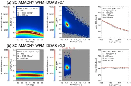
Fig. 5. Comparison of the O2-column ratio (Oret2 /Oref2 ) for SCIAMACHY WFM-DOAS version 2.1 (a) and 2.2 (b) using all data from the years 2003–2009. (a) The left panel shows a 2-D-histogram of the O2ratio as a function of the viewing zenith angle (VZA). The white curve is a quadratic fit. The middle panel shows a 2-D-histogram ofXCO2as a function of the scan-angle bias corrected O2ratio. The right panel showsXCO2averaged over scan-angle bias corrected O2ratio intervals. The red curve is a polynomial fit. (b) as in (a) but for WFM-DOAS version 2.2. The red lines in the left and middle panel indicate the new O2ratio thresholds (P1=0.95 andP2=1.1).
is determined from the US standard atmosphere O2column by accounting for the surface elevation variations in order to obtain the same O2ratio as used by Schneising et al. (2011). Heymann et al. (2012) showed that clouds with eCOD (effec-tive cloud optical depth defined as cloud fractional coverage times cloud optical depth) less than 0.1 may remain unde-tected. These undetected clouds can cause systematic errors, which are significant for the CO2surface flux inversion ap-plication. For this reason, we have also investigated to what extent a more restrictive O2ratio threshold can improve the quality of theXCO2data product.
A geometrical viewing geometry correction has been im-plemented for the O2and CO2 column in WFM-DOAS in order to correct for a scan-angle dependent air-mass factor (Buchwitz and Burrows, 2004). For this reason, the O2 ver-tical column ratio should be independent of the viewing ge-ometry. However, we found that the O2ratio exhibits a scan-angle dependent bias. In order to improve the geometrical correction, we correct for this bias using an empirical correc-tion. A quadratic function depending on the (signed) viewing zenith angle (VZA) (as defined by Heymann et al., 2012) was fitted to the O2ratio and used for the correction:
(Oret2 /Oref2 )cor=Oret2 /Oref2 +A2·(VZA−A3)2 (1) Oret2 corresponds to the retrieved and Oref2 to the reference O2column.A2is 3.26×10⁻⁵ 1(◦)2 andA3is−12.3
◦. These
values are adapted from the fit shown in the top left panel of Fig. 5. This figure shows the scan-angle dependency before the scan-angle bias correction of the O2ratio of WFMDv2.1 in the top left panel and after the scan-angle bias correction for WFMDv2.2 in the bottom left panel.
We use the scan-angle bias corrected O2 ratio for cloud filtering in the following way: If the O2 ratio of a ground pixel exceeds 1.1 or is smaller than 0.95, the ground pixel is flagged as cloudy. O2 ratios smaller than 1 indicate a light path shortening (e.g. due to cloud shielding), whereas O2 ra-tios larger than 1 indicate a light path lengthening (e.g. due to multiple scattering). For this reason, we increase the lower threshold of 0.9 of WFMDv2.1 to 0.95 and we added the up-per threshold of 1.1.
Fig. 6. Locations analysed in this study. The red diamonds show the locations used for the comparison of WFMD versions 2.1 and 2.2 with FTS measurements. The blue diamonds show the locations used for the determination of the monthly regional-scale scatter of the data in Sect. 4.2.
Table 2. Scatter of the WFMDv2.1 and v2.2 XCO2data products at several locations and overall (MEAN).
Monthly regional-scale scatter of the data
Location Country Lat [◦] Lon [◦] WFMDv2.1 WFMDv2.2 abs [ppm] rel [%] abs [ppm] rel [%]
Bialystok Poland 53.2 23.0 6.09 1.59 4.61 1.21 Khromtau Kazakhstan 50.3 58.5 9.23 2.43 4.68 1.23 Orleans France 48.0 2.1 6.28 1.64 4.48 1.17 Garmisch Germany 47.5 11.1 8.09 2.14 5.56 1.46 Park Falls USA 46.0 −90.3 7.65 2.01 5.29 1.39 Lamont USA 36.6 −97.5 7.56 1.99 4.01 1.05 Tazirbu Libya 25.7 21.4 4.95 1.30 3.48 0.91 Lubumbashi Congo −11.7 27.5 9.09 2.39 4.68 1.23 Darwin Australia −12.4 130.9 7.20 1.88 3.80 1.00 Brasilia Brazil −15.8 −47.9 8.26 2.16 4.52 1.19 Wollongong Australia −34.4 150.9 7.17 1.89 4.52 1.19
MEAN 7.42±1.29 1.95±0.34 4.51±0.60 1.18±0.16
SZA, surface albedos and optical depths. The reason for this dependency is different light paths in the retrieval of the O2 and CO2 columns used spectral regions due to scatter-ing by aerosols and thin clouds. Therefore, we have investi-gated if a reference O2column obtained from ECMWF (Eu-ropean Centre for Medium-Range Weather Forecasts) sur-face pressure and used for the normalisation of the CO2 column improves the quality of the XCO2 data product. However, we find large regional patterns, a much larger
than scattering by aerosols and thin clouds can be neglected. We use a polynomial fitted to averagedXCO2and O2ratios: XCOc2=XCO2+B1+B2·z+B3·z2 (2)
z=((Oret2 /Oref2 )cor−1).
HereB1is−0.8 ppm and accounts for a global offset.B2is 137 ppm andB3is−362 ppm. The fit parameters shown in Fig. 5 top-right are used for this correction. The bottom-right and mid-panels in this figure show the resulting dependency ofXCO2on the O2ratio after applying the improved filter method. As can be seen, the stricter O2ratio thresholds re-move unrealistic high and low values ofXCO2 and the re-maining O2ratio dependent bias inXCO2is very small. 4.2 Single measurement precision
Heymann et al. (2012) determined the monthly regional-scale scatter of the SCIAMACHY WFMDv2.1XCO2data product of about 7.42±1.29 ppm. We have used the same method to determine this value for the new version 2.2 data product.
The scatter is derived as follows: we compute the stan-dard deviation of allXCO2measurements within a radius of 350 km around several locations for each month. The loca-tions used for this assessment are shown in Fig. 6 and their latitudes and longitudes are listed in Table 2. We have se-lected the same locations as used by Heymann et al. (2012). For these locations sufficientXCO2 data are available and they are distributed over all continents covered by the data. The mean of the monthly standard deviations is derived for all locations. The overall value of the scatter is the mean of the scatter of all locations. This value is not only de-termined by instrumental and retrieval noise. Atmospheric
XCO2 variability and systematic errors can also affect this value (note that the seasonal cycle is filtered out by using the standard deviations of the monthly data). However, the com-puted monthly regional-scale scatter of the data can be re-garded as an upper limit of the single measurement precision. The standard deviations of WFMDv2.1 and WFMDv2.2
XCO2 are listed in Table 2. As can be seen, the standard deviation is smaller for version 2.2. The monthly regional-scale scatter is reduced to 4.51±0.60 ppm for WFMDv2.2 compared to 7.42±1.29 ppm for WFMDv2.1.
In addition, we estimated the single measurement preci-sion using the same approach as used in the publication of Schneising et al. (2011). They estimated the precision by averaging daily standard deviations of the retrievedXCO2 for 8 locations distributed around the globe. This estima-tion shows a reducestima-tion of the single measurement precision from 5.4 ppm (1.4 %) of WFMDv2.1 to 3.8 ppm (1 %) of WFMDv2.2.
5 Data sets used for comparison
In this section, the data sets used for the comparison with the new SCIAMACHY WFM-DOASXCO2version 2.2 as well as with the previous version 2.1 data product are briefly described.
5.1 TCCON
We use the independent measurements from the ground-based Fourier transform spectrometers (FTS) of TCCON (Total Carbon Column Observing Network) for the valida-tion of the SCIAMACHY WFMDv2.2XCO2data product. TCCON is a global network of ground-based FTS instru-ments and provides measureinstru-ments of CO2 and other green-house gases (Wunch et al., 2011). The FTS measurements are the most important validation source for measurements from satellite instruments like SCIAMACHY and GOSAT and fu-ture satellite missions like OCO-2 (Crisp et al., 2004; B¨osch et al., 2011) and CarbonSat (Bovensmann et al., 2010). A sta-ble and robust commercial high-resolution FTS, the Bruker IFS 125/HR, is used as standard instrument and common data processing and analysis software is utilised to determine
XCO2with a high accuracy of approximately 0.2 % (Wunch et al., 2011).
We obtained the FTS data from the TCCON website (http://www.tccon.caltech.edu) and use monthly means in this study.
5.2 CarbonTracker
For a global comparison of the SCIAMACHY WFM-DOAS v2.1 and v2.2XCO2, we use NOAA’s global CO2modelling and assimilation system CarbonTracker. CarbonTracker has been developed to estimate the global atmospheric CO2 dis-tribution and the CO2surface fluxes (Peters et al., 2007). Car-bonTracker assimilates precise and accurate measurements of NOAA’s greenhouse gas air sampling network. Version 2010 of CarbonTracker for the years 2003–2009 has been downloaded from http://carbontracker.noaa.gov. In order to obtain daily CarbonTrackerXCO2, the CarbonTracker CO2 vertical profiles have been vertically integrated after apply-ing the averagapply-ing kernels of the SCIAMACHY WFM-DOAS
XCO2retrieval algorithm. This daily CarbonTrackerXCO2 data set has been regridded on a latitude/longitude grid and sampled like the SCIAMACHY measurements.
6 Validation with TCCON FTS measurements
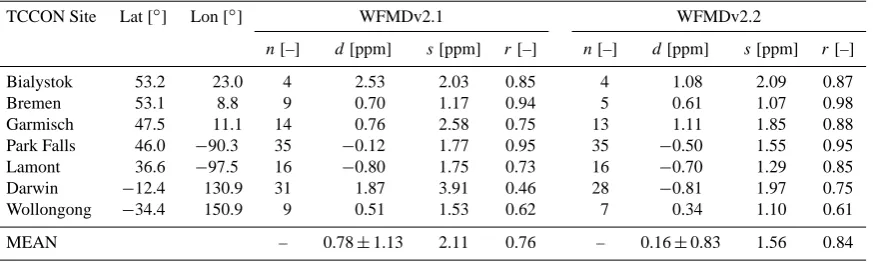
Table 3. Results of the comparison of WFMDv2.1 and v2.2XCO2data with ground based FTS measurements at various TCCON sites. The comparison is based on monthly data. Shown are the number of months used for the comparison (n), the mean difference to FTS (d), the standard deviation of the difference (s) and the correlation (r). In addition, the following quantities are given in the bottom row (MEAN): the averaged mean difference (global offset), the standard deviation of the mean differences (relative regional-scale accuracy), the mean standard deviation of the differences (monthly regional-scale precision) and the mean correlation.
TCCON Site Lat [◦] Lon [◦] WFMDv2.1 WFMDv2.2
n[–] d[ppm] s[ppm] r[–] n[–] d[ppm] s[ppm] r[–]
Bialystok 53.2 23.0 4 2.53 2.03 0.85 4 1.08 2.09 0.87 Bremen 53.1 8.8 9 0.70 1.17 0.94 5 0.61 1.07 0.98 Garmisch 47.5 11.1 14 0.76 2.58 0.75 13 1.11 1.85 0.88 Park Falls 46.0 −90.3 35 −0.12 1.77 0.95 35 −0.50 1.55 0.95 Lamont 36.6 −97.5 16 −0.80 1.75 0.73 16 −0.70 1.29 0.85 Darwin −12.4 130.9 31 1.87 3.91 0.46 28 −0.81 1.97 0.75 Wollongong −34.4 150.9 9 0.51 1.53 0.62 7 0.34 1.10 0.61
MEAN – 0.78±1.13 2.11 0.76 – 0.16±0.83 1.56 0.84
(Schneising et al., 2012). In this section, the result of this intercomparison are discussed.
6.1 Validation method
The validation of the WFMDv2.2 XCO2 is performed in the same way as described in the publication of Schneis-ing et al. (2012) for WFMDv2.1. This implies that monthly means for the time period 2003–2009 computed using a suf-ficiently large number of measurements within a radius of 500 km around the analysed TCCON sites (Bialystok, Bre-men, Garmisch, Park Falls, Lamont, Darwin and Wollon-gong) are used. The locations of the TCCON sites are shown in Fig. 6 and the corresponding latitudes and longitudes are listed in Table 3.
From the monthly time series of the satellite and FTS data statistical quantities are determined for every FTS site: the re-gional bias (d) (mean difference to FTS measurements), the mean standard deviation of the difference (s) and the linear correlation coefficient (r) with the FTS measurements. From these values we determine the offset, the monthly regional-scale precision (the mean standard deviation of the difference to FTS), the mean correlation and the regional-scale rela-tive accuracy (the standard deviation of the station-to-station biases).
The FTS and the satellite measurements provide infor-mation on the retrieved CO2column from different heights because of differing height sensitivities, as characterised by their averaging kernels. In order to compare these measurements, we use the comparison approach described by Rodgers (2000). The retrieved satellite and FTS CO2 columns have been adjusted to a common a priori profile. For this study, we use the same adjustment method as described by Reuter et al. (2011) and Schneising et al. (2012).
6.2 Validation results
The results of the comparison of the WFMDv2.1 and WFMDv2.2XCO2data product with the TCCON FTS mea-surements are shown in Fig. 7 and summarised in Table 3.
The comparison of WFMDv2.1XCO2with the FTS mea-surements for Darwin, Australia, shows a large monthly scat-ter of the data (7.2 ppm) and large differences to the FTS (3.9 ppm). This is improved for the new WFMDv2.2XCO2 data product. The scatter is reduced to 3.8 ppm. The large deviation to the FTS is improved by nearly a factor of 2 (from 3.9 ppm to 2.0 ppm). The improvement is also shown by a higher correlation (0.75) between the satellite and the FTS data.
Overall, the comparison of WFMDv2.2XCO2with FTS shows much better agreement than for WFMDv2.1. The monthly regional-scale precision has been improved from 2.1 ppm for WFMDv2.1 to 1.6 ppm for WFMDv2.2. The regional-scale relative accuracy has been improved from 1.1 ppm to 0.8 ppm and the mean correlation has been im-proved from 0.76 to 0.84.
These results show that the improved cloud filtering and correction method for WFMDv2.2 significantly improves the quality of theXCO2data product.
7 Comparison with CarbonTrackerXCO2
In addition to the comparison with the limited number of TCCON sites, we have also performed a comparison of WFMDv2.2XCO2with global model results using NOAA’s CarbonTracker.
a width of 20×20 (10◦×10◦) because some grid boxes do
not have sufficient data to remove the statistical error. The SCIAMACHY XCO2 maps also show that with the much stricter cloud filtering and correction method good cover-age of most land surfaces is achieved. There are however some gaps, e.g. Sahara and Himalaya, similar to WFMDv2.1. The maps of the SCIAMACHY and CarbonTrackerXCO2 also show the northern hemispherical terrestrial vegetation induced carbon uptake in summer as shown by higherXCO2 values in April–June compared to lower XCO2 values in July–September in 2003 and 2009. In addition, the increase of the global CO2concentration is seen by the higherXCO2 in 2009 compared to 2003. Both data sets show reasonable agreement. There are, however, also significant differences, e.g. over India and the Horn of Africa, which needs further investigation.
For a more quantitative investigation, we compared WFMDv2.2 with CarbonTrackerXCO2using hemispherical monthly means between 2003 and 2009. In order to inves-tigate if the improved cloud filtering and correction method reduces the difference to CarbonTracker, we compare with WFM-DOAS v2.1XCO2. However, it has to be noted that CarbonTracker is affected by errors of its own like, e.g. in-correct accounting for the vertical transport and the ageing of air and uncertainties in the biosphere fluxes (Basu et al., 2011).
Important parameters for the comparison are determined in the following way: the annual increase is determined by smoothing the time series with a twelve-month boxcar func-tion and computing the mean from the derivative of the smoothed time series. The seasonal cycle amplitude is deter-mined from a detrended time series between 2004 and 2008 by averaging the yearly difference of maximum and mini-mumXCO2 . The error of the increase and the amplitude is estimated by a bootstrap method (see Schneising et al., 2011). The correlation with CarbonTracker and the standard deviation of the difference to CarbonTracker has been deter-mined. In addition, the detrended correlation coefficient (r) to CarbonTracker is computed from the detrended time se-ries of WFMDv2.1 and WFMDv2.2 and is an indicator for (phase) shifts between the time series.
Figure 9 shows the result of this comparison. As can be seen, the scatter is reduced from 10.2 ppm for WFMDv2.1 to 5.8 ppm for WFMDv2.2 for the Northern Hemisphere and from 9.2 ppm to 4.6 ppm for the Southern Hemisphere. The correlation with CarbonTracker is for both WFM-DOAS ver-sions and for both hemispheres nearly the same. The standard deviation of the differences is slightly worse for the North-ern Hemisphere (from 1.3 ppm to 1.5 ppm) and slightly bet-ter for the Southern Hemisphere (from 1.3 ppm to 0.9 ppm). The annual increase, the seasonal cycle amplitude and the detrended correlation of the Northern Hemisphere are not changed significantly. The reason for the observed difference in the seasonal cycle amplitude can be an underestimation of the net ecosystem exchange (NEE) between the atmosphere
and the biosphere in the CASA (Carnegie-Ames-Stanford Approach) biosphere model which is used by CarbonTracker (Yang et al., 2007; Schneising et al., 2012; Keppel-Aleks et al., 2012; Messerschmidt et al., 2012). For the Southern Hemisphere, the annual increase of WFMDv2.2 is also not changed significantly. However, the seasonal cycle ampli-tude is lower for WFMDv2.2 and agrees better with Car-bonTracker compared to WFMDv2.1. The phase shift of the seasonal cycle of WFMDv2.1 shown by the detrended corre-lation of−0.19 was significantly improved for WFMDv2.2 shown by the detrended correlation of 0.72.
Overall, the SCIAMACHY WFM-DOAS v2.2XCO2data product shows much better agreements with CarbonTracker compared to WFMDv2.1.
8 Summary and conclusions
We have presented an improved version (WFMDv2.2) of the SCIAMACHY WFM-DOASXCO2retrieval algorithm. This algorithm utilises an improved cloud filtering and correc-tion method using the 1.4 µm water vapour absorpcorrec-tion and 0.76 µm O2-A bands to identify and select cloud free scenes. A new SCIAMACHY XCO2 data set covering the years 2003–2009 has been generated by using this new version. In order to validate the new XCO2 data product, we used ground-based FTS observations from TCCON.
The validation showed a significant improvement of the new SCIAMACHYXCO2data product (v2.2) in comparison to the previous product (v2.1). For example, the large time dependent deviation from the FTS measurements at Darwin was reduced from a standard deviation of 4 ppm to 2 ppm. The monthly regional-scale scatter of the data (defined as standard deviation of all monthly quality filteredXCO2 re-trievals within a radius of 350 km around various locations) was also improved typically by a factor of about 1.5. Over-all, the single measurement precision has been improved from 5.4 ppm for WFMDv2.1 to 3.8 ppm for WFMDv2.2, the monthly regional-scale precision has been improved from 2.1 ppm to 1.6 ppm, the regional-scale relative accuracy has been improved from 1.1 ppm to 0.8 ppm and the mean corre-lation has also been improved from 0.76 to 0.84.
In addition to the comparison with the limited number of TCCON sites, we also presented results of a comparison with NOAA’s global CO2modelling and assimilation system Car-bonTracker. The results of this comparison also showed sig-nificant improvements of the newXCO2data product espe-cially over the Southern Hemisphere (e.g. a reduction of the phase shift between the SCIAMACHY and CarbonTracker
XCO2).
Fig. 9. Comparison of SCIAMACHY WFM-DOAS version 2.1 (WFMDv2.1) and 2.2 (WFMDv2.2) with CarbonTrackerXCO2for the Northern (top) and Southern (bottom) Hemisphere for the years 2003–2009. CarbonTracker was sampled as WFMDv2.1 (@v2.1) for the comparison with WFMDv2.1 and sampled as WFMDv2.2 (@v2.2) for the comparison with WFMDv2.2. Top: The left panel shows the time series of monthly means of WFMDv2.1 (black diamonds), WFMDv2.2 (blue crosses) and CarbonTracker (red triangles)XCO2and the difference to CarbonTracker for the Northern Hemisphere. The shaded areas represent the monthly standard deviations of WFMDv2.1 (grey), WFMDv2.2 (light blue) and CarbonTracker (red). In addition, the averaged monthly standard deviation, the correlation with CarbonTracker and the standard deviation of the difference to CarbonTracker are shown. The right panel shows the detrended time series. Furthermore, the annual increase, the seasonal cycle amplitude and the detrended correlation (correlation between the detrended satellite time series and CarbonTracker) are shown. Bottom: as in top panels but for the Southern Hemisphere.
set is available on request from http://www.iup.uni-bremen. de/sciamachy/NIR NADIR WFM DOAS/.
Acknowledgements. CarbonTracker version 2010 data were pro-vided by NOAA ESRL, Boulder, Colorado, USA, via the web-site at http://carbontracker.noaa.gov. We thank ECMWF for provid-ing the meteorological data. The TCCON data were obtained from the TCCON Data Archive, operated by the California Institute of
The Garmisch TCCON activities have been funded by the ESA GHG-CCI project via subcontract with the University of Bremen and by the EC within the INGOS project.
The Darwin and Wollongong TCCON sites are funded by NASA grants NAG5-12247 and NNG05-GD07G and the Australian Re-search Council, DP0879468 and LP0562346. We are grateful to the DOE ARM program for technical support in Darwin.
The Park Falls and Lamont TCCON stations are funded by NASA grants NNX11AG01G, NAG5-12247, NNG05-GD07G, and NASA’s Orbiting Carbon Observatory Program. We are grateful to the DOE ARM program for technical support in Lamont and Jeff Ayers for technical support in Park Falls.
The TCCON site at Bialystok is financially supported by the Senate of Bremen and the EU projects IMECC and GEOmon. We acknowledge maintenance and logistical work provided by AeroMeteo Service (Bialystok) and RAMCES team at LSCE (Gif-sur-Yvette, France).
Edited by: T. von Clarmann
References
Barkley, M. P., Frieß, U., and Monks, P. S.: Measuring atmospheric CO2 from space using Full Spectral Initiation (FSI) WFM-DOAS, Atmos. Chem. Phys., 6, 3517–3534, doi:10.5194/acp-6-3517-2006, 2006a.
Barkley, M. P., Monks, P. S., Hewitt, A. J., Machida, T., Desai, A., Vinnichenko, N., Nakazawa, T., Yu Arshinov, M., Fedoseev, N., and Watai, T.: Assessing the near surface sensitivity of SCIA-MACHY atmospheric CO2retrieved using (FSI) WFM-DOAS, Atmos. Chem. Phys., 7, 3597–3619, doi:10.5194/acp-7-3597-2007, 2007.
Basu, S., Houweling, S., Peters, W., Sweeney, C., Machida, T., Maksyutov, S., Patra, P. K., Saito, R., Chevallier, F., Niwa, Y., Matsueda, H., and Sawa, Y.: The seasonal cy-cle amplitude of total column CO2: factors behind the model-observation mismatch, J. Geophys. Res., 116, D23306, doi:10.1029/2011JD016124, 2011.
B¨osch, H., Toon, G. C., Sen, B., Washenfelder, R. A., Wennberg, P. O., Buchwitz, M., de Beek, R., Burrows, J. P., Crisp, D., Christi, M., Connor, B. J., Natraj, V., and Yung, Y. L.: Space-based near-infrared CO2measurements: testing the Orbit-ing Carbon Observatory retrieval algorithm and validation con-cept using SCIAMACHY observations over Park Falls, Wiscon-sin, J. Geophys. Res., 111, D23302, doi:10.1029/2006JD007080, 2006.
B¨osch, H., Baker, D., Connor, B., Crisp, D., and Miller, C.: Global characterization of CO2 column retrievals from shortwave-infrared satellite observations of the Orbiting Car-bon Observatory-2 mission, Remote Sens., 3, 270–304, doi:10.3390/rs3020270, 2011.
Bovensmann, H., Burrows, J. P., Buchwitz, M., Frerick, J., No¨el, S., Rozanov, V. V., Chance, K. V., and Goede, A.: SCIAMACHY – mission objectives and measurement modes, J. Atmos. Sci., 56, 127–150, 1999.
Bovensmann, H., Buchwitz, M., Burrows, J. P., Reuter, M., Krings, T., Gerilowski, K., Schneising, O., Heymann, J., Tret-ner, A., and Erzinger, J.: A remote sensing technique for global monitoring of power plant CO2emissions from space and related applications, Atmos. Meas. Tech., 3, 781–811, doi:10.5194/amt-3-781-2010, 2010.
Buchwitz, M. and Burrows, J. P.: Retrieval of CH4, CO, and CO2 total column amounts from SCIAMACHY near-infrared nadir spectra: retrieval algorithm and first results, in: Remote Sensing of Clouds and the Atmosphere VIII, edited by: Sch¨afer, K. P., Com`eron, A., Carleer, M. R., and Picard, R. H., Proc. SPIE, 5235, 375–388, 2004.
Buchwitz, M., Rozanov, V. V., and Burrows, J. P.: A near-infrared optimized DOAS method for the fast global retrieval of atmo-spheric CH4, CO, CO2, H2O, and N2O total column amounts from SCIAMACHY Envisat-1 nadir radiances, J. Geophys. Res., 105, 15231–15245, 2000.
Buchwitz, M., de Beek, R., No¨el, S., Burrows, J. P., Bovens-mann, H., Schneising, O., Khlystova, I., Bruns, M., Bremer, H., Bergamaschi, P., K¨orner, S., and Heimann, M.: Atmospheric carbon gases retrieved from SCIAMACHY by WFM-DOAS: version 0.5 CO and CH4 and impact of calibration improve-ments on CO2 retrieval, Atmos. Chem. Phys., 6, 2727–2751, doi:10.5194/acp-6-2727-2006, 2006.
Buchwitz, M., Schneising, O., Burrows, J. P., Bovensmann, H., Reuter, M., and Notholt, J.: First direct observation of the at-mospheric CO2year-to-year increase from space, Atmos. Chem. Phys., 7, 4249–4256, doi:10.5194/acp-7-4249-2007, 2007. Burrows, J. P., H¨olzle, E., Goede, A. P. H., Visser, H., and
Fricke, W.: SCIAMACHY – Scanning Imaging Absorption Spectrometer for Atmospheric Chartography, Acta Astronaut., 35, 445–451, 1995.
Butz, A., Hasekamp, O. P., Frankenberg, C., and Aben, I.: Retrievals of atmospheric CO2from simulated space-borne measurements of backscatteres near-infrared sunlight: accounting for aerosol ef-fects, Appl. Opt., 48, 3322–3336, 2009.
Chevallier, F., Br´eon, F.-M., and Rayner, P. J.: Contribution of the Orbiting Carbon Observatory to the estimation of CO2 sources and sinks: theoretical study in a variational data assimilation framework, J. Geophys. Res., 112, D09307, doi:10.1029/2006JD007375, 2007.
Crisp, D., Atlas, R. M., Br´eon, F.-M., Brown, L. R., Bur-rows, J. P., Ciais, P., Connor, B. J., Doney, S. C., Fung, I. Y., Jacob, D. J., Miller, C. E., O’Brien, D., Paw-son, S., RanderPaw-son, J. T., Rayner, P., Salawitch, R. S., Sander, S. P., Sen, B., Stephens, G. L., Tans, P. P., Toon, G. C., Wennberg, P. O., Wofsy, S. C., Yung, Y. L., Kuang, Z., Chu-dasama, B., Sprague, G., Weiss, P., Pollock, R., Kenyon, D., and Schroll, S.: The Orbiting Carbon Observatory (OCO) mission, Adv. Space Res., 34, 700–709, 2004.
Gao, B.-C., Goetz, A. F. H., and Wiscombe, W. J.: Cirrus cloud detection from airborne imaging spectromter data using the 1.38 µm water vapor band, Geophys. Res. Lett., 20, 301–304, 1993.
Houweling, S., Breon, F.-M., Aben, I., R¨odenbeck, C., Gloor, M., Heimann, M., and Ciais, P.: Inverse modeling of CO2sources and sinks using satellite data: a synthetic inter-comparison of mea-surement techniques and their performance as a function of space and time, Atmos. Chem. Phys., 4, 523–538, doi:10.5194/acp-4-523-2004, 2004.
Houweling, S., Hartmann, W., Aben, I., Schrijver, H., Skidmore, J., Roelofs, G.-J., and Breon, F.-M.: Evidence of systematic errors in SCIAMACHY-observed CO2due to aerosols, Atmos. Chem. Phys., 5, 3003–3013, doi:10.5194/acp-5-3003-2005, 2005. Keppel-Aleks, G., Wennberg, P. O., Washenfelder, R. A., Wunch,
D., Schneider, T., Toon, G. C., Andres, R. J., Blavier, J.-F., Con-nor, B., Davis, K. J., Desai, A. R., Messerschmidt, J., Notholt, J., Roehl, C. M., Sherlock, V., Stephens, B. B., Vay, S. A., and Wofsy, S. C.: The imprint of surface fluxes and transport on vari-ations in total column carbon dioxide, Biogeosciences, 9, 875– 891, doi:10.5194/bg-9-875-2012, 2012.
Kuze, A., Suto, H., Nakajima, M., and Hamazaki, T.: Thermal and near infrared sensor for carbon observation Fourier-transform spectrometer on the Greenhouse Gases Observing Satellite for greenhouse gases monitoring, Appl. Optics, 48, 6716–6733, 2009.
Messerschmidt, J., Parazoo, N., Deutscher, N. M., Roehl, C., Warneke, T., Wennberg, P. O., and Wunch, D.: Evaluation of atmosphere-biosphere exchange estimations with TCCON mea-surements, Atmos. Chem. Phys. Discuss., 12, 12759–12800, doi:10.5194/acpd-12-12759-2012, 2012.
Miller, C. E., Crisp, D., DeCola, P. L., Olsen, S. C., Rander-son, J. T., Michalak, A. M., Alkhaled, A., Rayner, P., Ja-cob, D. J., Suntharalingam, P., Jones, D. B. A., Denning, A. S., Nicholls, M. E., Doney, S. C., Pawson, S., Boesch, H., Con-nor, B. J., Fung, I. Y., O’Brien, D., Salawitch, R. J., Sander, S. P., Sen, B., Tans, P., Toon, G. C., Wennberg, P. O., Wofsy, S. C., Yung, Y. L., and Law, R. M.: Precision requirements for space-based XCO2 data, J. Geophys. Res., 112, D10314, doi:10.1029/2006JD007659, 2007.
Morino, I., Uchino, O., Inoue, M., Yoshida, Y., Yokota, T., Wennberg, P. O., Toon, G. C., Wunch, D., Roehl, C. M., Notholt, J., Warneke, T., Messerschmidt, J., Griffith, D. W. T., Deutscher, N. M., Sherlock, V., Connor, B., Robinson, J., Suss-mann, R., and Rettinger, M.: Preliminary validation of column-averaged volume mixing ratios of carbon dioxide and methane retrieved from GOSAT short-wavelength infrared spectra, At-mos. Meas. Tech., 4, 1061–1076, doi:10.5194/amt-4-1061-2011, 2011.
O’Dell, C. W., Connor, B., B¨osch, H., O’Brien, D., Frankenberg, C., Castano, R., Christi, M., Eldering, D., Fisher, B., Gunson, M., McDuffie, J., Miller, C. E., Natraj, V., Oyafuso, F., Polon-sky, I., Smyth, M., Taylor, T., Toon, G. C., Wennberg, P. O., and Wunch, D.: The ACOS CO2retrieval algorithm - Part 1: Descrip-tion and validaDescrip-tion against synthetic observaDescrip-tions, Atmos. Meas. Tech., 5, 99–121, doi:10.5194/amt-5-99-2012, 2012.
Oshchepkov, S., Bril, A., and Yokota, T.: PPDF-based method to account for atmospheric light scattering in observations of car-bon dioxide from space, J. Geophys. Res.-Atmos., 113, D23210, doi:10.1029/2008JD010061, 2008.
Peters, W., Jacobson, A. R., Sweeney, C., Andrews, A. E., Con-way, T. J., Masarie, K., Miller, J. B., Bruhwiler, L. M. P., Petron, G., Hirsch, A. I., Worthy, D. E. J., van der Werf, G. R.,
Randerson, J. T., Wennberg, P. O., Krol, M. C., and Tans, P. P.: An atmospheric perspective on North American carbon diox-ide exchange: CarbonTracker, Proc. Natl. Acad. Sci. USA, 104, 18925–18930, doi:10.1073/pnas.0708986104, 2007.
Rayner, P. J. and O’Brien, D. M.: The utility of remotely sensed CO2 concentration data in surface inversions, Geo-phys. Res. Lett., 28, 175–178, 2001.
Reuter, M., Bovensmann, H., Buchwitz, M., Burrows, J. P., Connor, B. J., Deutscher, N. M., Griffith, D. W. T., Hey-mann, J., Keppel-Aleks, G., Messerschmidt, J., Notholt, J., Petri, C., Robinson, J., Schneising, O., Sherlock, V., Velazco, V., Warneke, T., Wennberg, P. O., and Wunch, D.: Retrieval of atmospheric CO2 with enhanced accuracy and precision from SCIAMACHY: Validation with FTS measurements and com-parison with model results, J. Geophys. Res., 116, D04301, doi:10.1029/2010JD015047, 2011.
Rodgers, C. D.: Inverse Methods for Atmospheric Sounding: The-ory and Practice, World Scientific Publishing, Singapore, 2000. Saitoh, N., Imasu, R., Ota, Y., and Niwa, Y.: CO2 retrieval
algo-rithm for the thermal infrared spectra of the Greenhouse Gases Observing Satellite: potential of retrieving CO2vertical profile from high-resolution FTS sensor, J. Geophys. Res., 114, D17305, doi:10.1029/2008JD011500, 2009.
Schneising, O., Buchwitz, M., Burrows, J. P., Bovensmann, H., Reuter, M., Notholt, J., Macatangay, R., and Warneke, T.: Three years of greenhouse gas column-averaged dry air mole fractions retrieved from satellite – Part 1: Carbon dioxide, Atmos. Chem. Phys., 8, 3827–3853, doi:10.5194/acp-8-3827-2008, 2008. Schneising, O., Buchwitz, M., Reuter, M., Heymann, J.,
Bovens-mann, H., and Burrows, J. P.: Long-term analysis of car-bon dioxide and methane column-averaged mole fractions re-trieved from SCIAMACHY, Atmos. Chem. Phys., 11, 2863– 2880, doi:10.5194/acp-11-2863-2011, 2011.
Schneising, O., Bergamaschi, P., Bovensmann, H., Buchwitz, M., Burrows, J. P., Deutscher, N. M., Griffith, D. W. T., Heymann, J., Macatangay, R., Messerschmidt, J., Notholt, J., Rettinger, M., Reuter, M., Sussmann, R., Velazco, V. A., Warneke, T., Wennberg, P. O., and Wunch, D.: Atmospheric greenhouse gases retrieved from SCIAMACHY: comparison to ground-based FTS measurements and model results, Atmos. Chem. Phys., 12, 1527–1540, doi:10.5194/acp-12-1527-2012, 2012.
Stephens, B. B., Gurney, K. R., Tans, P. P., Sweeney, C., Pe-ters, W., Bruhwiler, L., Ciais, P., Ramonet, M., Bousquet, P., Nakazawa, T., Aoki, S., Machida, T., Inoue, G., Vinnichenko, N., Lloyd, J., Jordan, A., Heimann, M., Shibistova, O., Langen-felds, R. L., Steele, L. P., Francey, R. J., and Denning, A. S.: Weak northern and strong tropical land carbon uptake from ver-tical profiles of atmospheric CO2, Science, 316, 1732–1735, doi:10.1126/science.1137004, 2007.
Tilstra, L. G., de Graaf, M., Aben, I., and Stammes, P.: Analysis of 5 years of SCIAMACHY absorbing aerosol index data, Pro-ceedings ENVISAT Symposium, Montreux, Switzerland, ESA Special Publication SP-636, 2007.
Yang, Z., Washenfelder, R. A., Keppel-Aleks, G., Krakauer, N. Y., Randerson, J. T., Tans, P. P., Sweeney, C., and Wennberg, P. O.: New constraints on Northern Hemisphere growing season net flux, Geophys. Res. Lett., 34, L12807, doi:10.1029/2007GL029742, 2007.
Yokota, T., Oguma, H., Morino, I., and Inoue, G.: A nadir look-ing SWIR sensor to monitor CO2column density for Japanese GOSAT project, Proceedings of the twenty-fourth international symposium on space technology and science, Miyazaki: Japan Society for Aeronautical and Space Sciences and ISTS, 887–889, 2004.
Yoshida, J., Kawashima, T., Ishida, J., Kuze, A., Suto, H., Sh-iomi, K., and Nakajima, M.: GOSAT/TANSO: Instrument Design and Level 1 Product Processing Algorithms, Fourier Transform Spectroscopy, OSA Technical Digest (CD) (Optical Society of America, 2011), paper JPDP1, available at: http: //www.opticsinfobase.org/abstract.cfm?URI=FTS-2011-JPDP1 (last access: June 2012), 2011a.