www.clim-past.net/6/445/2010/ doi:10.5194/cp-6-445-2010
© Author(s) 2010. CC Attribution 3.0 License.
Climate
of the Past
Influence of solar variability, CO
2
and orbital forcing between 1000
and 1850 AD in the IPSLCM4 model
J. Servonnat1, P. Yiou1, M. Khodri2, D. Swingedouw1,3, and S. Denvil4
1Laboratoire des Sciences du Climat et de l’Environnement (LSCE), UMR 8212 CEA-CNRS-UVSQ, Orme des Merisiers, 91191 Gif-sur-Yvette cedex, France
2Laboratoire d’Oc´eanographie et du Climat: Exp´erimentation et Approches Num´eriques (LOCEAN), 4 place Jussieu, 75252 Paris Cedex 05, France
3Centre Europ´een de Recherche et de Formation Avanc´ee en Calcul Scientifique, 42 avenue Gaspard Coriolis, 31057 Toulouse, France
4Institut Pierre Simon Laplace, 4 place Jussieu, 75252 Paris Cedex 05, France Received: 11 March 2010 – Published in Clim. Past Discuss.: 7 April 2010 Revised: 5 July 2010 – Accepted: 15 July 2010 – Published: 22 July 2010
Abstract. Studying the climate of the last millennium gives the possibility to deal with a relatively well-documented cli-mate essentially driven by natural forcings. We have per-formed two simulations with the IPSLCM4 climate model to evaluate the impact of Total Solar Irradiance (TSI), CO2 and orbital forcing on secular temperature variability during the preindustrial part of the last millennium. The Northern Hemisphere (NH) temperature of the simulation reproduces the amplitude of the NH temperature reconstructions over the last millennium. Using a linear statistical decomposition we evaluated that TSI and CO2 have similar contributions to secular temperature variability between 1425 and 1850 AD. They generate a temperature minimum comparable to the Little Ice Age shown by the temperature reconstructions. Solar forcing explains∼80% of the NH temperature variabil-ity during the first part of the millennium (1000–1425 AD) including the Medieval Climate Anomaly (MCA). It is re-sponsible for a warm period which occurs two centuries later than in the reconstructions. This mismatch implies that the secular variability during the MCA is not fully explained by the response of the model to the TSI reconstruction.
With a signal-noise ratio (SNR) estimate we found that the temperature signal of the forced simulation is signifi-cantly different from internal variability over area wider than ∼5.106km2, i.e. approximately the extent of Europe. Orbital forcing plays a significant role in latitudes higher than 65◦N
in summer and supports the conclusions of a recent study
Correspondence to: J. Servonnat
on an Arctic temperature reconstruction over past two mil-lennia. The forced variability represents at least half of the temperature signal on only∼30% of the surface of the globe. This study suggests that regional reconstructions of the tem-perature between 1000 and 1850 AD are likely to show weak signatures of solar, CO2and orbital forcings compared to in-ternal variability.
1 Introduction
The study of the last millennium climate has considerably increased during the last decades because it replaces the evo-lution of the global temperature for the last fifty years in a multi-centennial context, providing the necessary hindsight for a more comprehensive assessment of the recent climatic change. Studying this period gives the possibility to explore a relatively well-documented climate and weakly affected by anthropogenic greenhouse gases (GHGs). Before the indus-trial era, natural forcings such as volcanic aerosols and solar variability have likely dominated the forced variability of the Earth climate (Rind, 2002; Bauer et al., 2003; Bertrand et al., 2002; Mann et al., 1998; Robock, 2000; Hegerl et al., 2007; Crowley, 2000; Gerber et al., 2003; Jones and Mann, 2004). Several temperature reconstructions covering differ-ent areas of the globe are now available, ranging from multi-decadal to seasonal time scale. They were obtained from dif-ferent proxy data such as tree rings (Briffa et al., 2004; Cook et al., 2002; Esper et al., 2002; D’Arrigo et al., 2006; Os-born et al., 2006), fossil pollen (Bjune et al., 2004; Larocque and Hall, 2004), ice cores (Jouzel et al., 2001; Vinther et al.,
446 J. Servonnat et al.: Influence of solar variability, CO2and orbital forcing 2008), lake sediments (Hu et al., 2001; McKay et al., 2008),
boreholes (Gonzalez-Rouco et al., 2003a), speleothems (Tan et al., 2003; Mangini et al., 2005) and historical documents (Brazdil et al., 2005). This important amount of data has been used to perform empirical reconstructions of Northern Hemisphere (NH) surface temperature over the last millen-nium, relying on various methods to extract the hemispheric signal (Mann et al., 2008; Ammann and Wahl, 2007; Crow-ley and Lowery, 2000; Moberg et al., 2005; Hegerl et al., 2007). Those reconstructions carry however important un-certainties due to the calibration method, the type of proxy used and the reconstruction algorithm (Juckes et al., 2007; Mann et al., 2008). Due to these sources of uncertainties, robust conclusions regarding temperature variability for the past 1000 years have to be drawn by confronting as much re-constructions as possible. In the Southern Hemisphere proxy data are still too sparse to produce robust hemispherical tem-perature reconstructions (Juckes et al., 2007; Mann et al., 2008).
This increasingly documented period displays prominent climatic features for the last millennium such as the so-called Medieval Climate Anomaly (MCA, firstly introduced by (Lamb, 1965) as the “Medieval Warm Epoch”) and the Little Ice Age (LIA hereafter; Matthes, 1939). Those two periods have emerged from historical documents relating ex-ceptional conditions for agriculture for the former, or glaciers growing down in valleys for the latter. One main question concerning these identified periods is the extent to which they are global (or at least hemispherical) or local phenomenon (Bradley et al., 2003; Crowley and Lowery, 2000). It ap-pears that those episodes described in Europe are not al-ways present in all temperature reconstructions around the globe. The warmest and coldest periods of two time series can present asynchronous occurrence and differ in amplitude when comparing one region to another (Jones and Mann, 2004), although those differences can depend on the recon-struction methods (Esper and Frank, 2009). Nevertheless, at hemispherical scale the different reconstructions seem to converge toward a relatively warm period at the beginning of the last millennium, between 900 and 1300 AD, followed by a slow decrease in temperature reaching a minimum between 1600 and 1900 AD.
Climate models have been used to study the factors that could have been responsible for such climate evolution over the last millennium. Numerous modelling experiments with different levels of model complexity such as Energy Bal-ance Models (EBM), Earth system Models of Intermediate Complexity (EMIC) and General Circulation Models (GCM) have been carried out to assess this variability (Jansen et al., 2007). Those studies show that solar variability and vol-canic aerosols are the prominent drivers of the climate be-tween 1000 and 1850 AD at hemispherical scale. (Crowley, 2000) evaluated the role of both forcings during the preindus-trial era using an Energy Balance Model and showed that the low frequency variability over this period is mainly attributed
to solar variability, whereas volcanic forcing is dominant on decadal to interdecadal time scales. Same conclusions were found by (Bertrand et al., 2002) with the two-dimensional sector averaged global climate model of Louvain-la-Neuve and by (Goosse and Renssen, 2004) with the ECBilt-CLIO model. But when focusing on Europe with the same set of simulations, (Goosse et al., 2006) highlighted that land use could be in a large amount responsible for the decrease in temperature between the MWP and the LIA.
Detection and attribution methods on the last millennium climate give more moderated conclusions. Volcanic erup-tions are clearly discriminated by their cooling effect at a global scale, while the signature of solar variability on NH temperature reconstructions before 1850 AD is more subtle, and yields the same magnitude as the response to GHGs (Hegerl et al., 2003, 2007). Internal variability due to non-linear processes can be comparatively large especially at local scale, as shown by (Goosse et al., 2006). Using a 10 000 years EMIC with constant forcings (Hunt, 2006) found that internal processes of the model could not produce events similar to the MCA or the LIA at the hemispherical scale.
The role of the sun on climate variability during the last millennium remains unclear because of uncertainties of To-tal Solar Irradiance (TSI) past variations. For the period pre-ceding the beginning of satellites measurements (1979), the TSI is typically inferred from proxy data such as measure-ments of cosmogenic isotopes, mainly14C in tree rings and 10Be in ice cores (Bard et al., 2000; Muscheler et al., 2004, 2007), or observations of the Group Sunspot Number (GSN) back until 1610 (Lean et al., 1995; Krivova et al., 2007). The former is found in long archives such as ice cores or tree rings allowing to go further back in time than the GSN which displays however higher temporal resolution and is able to catch the 11-year Schwabe cycle associated to sun spots. The main TSI oscillations such as the Sp¨orer (∼1475 AD), Maunder (∼1700 AD) and Dalton (∼1800 AD) Min-ima are relatively well dated and constrained in proxy recon-structions, but their conversion into TSI values carries im-portant uncertainties (Bard et al., 2000). The amplitude of TSI secular variability is thus still under debate (Frohlich, 2009; Foukal et al., 2006; Frohlich and Lean, 2004). A decrease of about 0.25% of TSI during the Maunder Min-imum relative to present day value produces realistic am-plitude of the Northern Hemisphere temperature variability in climate models (Ammann et al., 2007). However, recent progress in solar physics (Foukal et al., 2004; Solanki and Krivova, 2006) shows that multidecadal to secular TSI vari-ability should mainly be due to sun-spots and faculae, which implies amplitude of TSI variations between the Maunder Minimum and present day value (last thirty years mean) of around 0.1%.
millennium to focus on the secular variability of the tem-perature, from the global scale to the grid point. We anal-yse the temperature response in two millennium-long climate simulations achieved with the coupled model developed at the Institut Pierre-Simon Laplace (IPSL): one with constant preindustrial boundary conditions, and one driven by a TSI reconstruction, GHGs concentrations and changes in orbital parameters between 1000 and 2000 AD. The contribution of each forcings on the simulated temperature variability is evaluated with a statistical decomposition of the temperature signal allowing a quantified estimation of the forced variabil-ity from the local to the global scale.
In Sect. 2, we describe the experimental design, the cli-mate model and the forcings used. Section 3 presents the analysis of the Northern Hemisphere surface temperature in both simulations and a comparison with temperature recon-structions, fed by an evaluation of the contribution of each forcing to the temperature variability in the forced simula-tion. In Sect. 4 we use a signal-to-noise ratio to compare the forced model response with the model internal variabil-ity, from the global to the local scale. This work ends in Sect. 5 with the discussion and conclusion.
2 Experimental design
We used the fully coupled climate model developed at the Institut Pierre-Simon Laplace, IPSLCM4 v2 (Marti et al., 2006). This model is composed of the LMDz4 atmosphere GCM (Hourdin et al., 2006), the OPA8.2 ocean model (Madec et al., 1998), the LIM2 sea-ice model (Fichefet and Maqueda, 1997) and ORCHIDEE 1.9.1 for continental sur-faces (Krinner et al., 2005). The coupling between the dif-ferent parts is done by OASIS (Valcke et al., 2000). The resolution in the atmosphere is 96×71×19, i.e. 3.75◦in
lon-gitude, 2.5◦ in latitude, and 19 vertical levels. The ocean
and sea-ice are implemented on the ORCA2 grid (averaged horizontal resolution∼2◦, refined to 0.5◦around the equator, 31 vertical levels). For both runs, the vegetation was set to a modern climatology from satellite observation (Myneni et al., 1997).
We ran a 110 years spin up with preindustrial GHGs con-centrations and tropospheric aerosols. The last year of the spin up is the initial state for both millennium-long simula-tions. The first one is a 1000-year control simulation (CTRL) with the same preindustrial boundary conditions as the spin up. The surface temperature of CTRL presents a weak drift during the first 100 years (−0.11◦C/100 yrs), and remains
stable during the following 900 years (10−3◦C/100 yrs). The
total heat content of the first 300 m of the ocean increases slowly during 600 yrs (∼0.9%), and then becomes stable, re-flecting the longer time needed for the thermal adjustment of the ocean.
The second simulation (SGI, for Solar, Greenhouse gases and Insolation) was forced with reconstructions of Total
So-lar Irradiance variations, GHGs concentrations and changes in orbital parameters covering the last millennium, from 1000 to 2000 AD. We chose the TSI reconstruction provided by (Crowley, 2000) (Fig. 1a) which combines one record derived from cosmogenic nuclides flux estimates (Bard et al., 2000) and another one inferred from sunspots observa-tions (Lean et al., 1995). The resulting amplitude of the TSI changes between the Maunder Minimum and present day values reaches 0.25% while capturing the decadal variability of sunspot cycles. The associated mean radiative forcing in Fig. 1a is estimated by dividing the TSI by four (distribution of the top of atmosphere flux on Earth surface), and multi-plied by the Earth’s albedo (∼0.7). We used the same recon-structions for well-mixed GHGs concentrations as those used in the fourth assessment report of the Fourth Intergovernmen-tal Panel on Climate Change (Jansen et al., 2007) for simu-lations of the climate of the last millennium. Only CO2 con-centration varies significantly before 1850 AD (Frank et al., 2010; Scheffer et al., 2006). The radiative forcing associated with changes in CO2 concentration in Fig. 1a is estimated with the equation of (Myhre et al., 1998). This equation gives a good estimate of the first order radiative forcing of CO2in the IPSL model (Dufresne, personal communication, 2009). Tropospheric aerosols concentrations are kept constant be-fore 1850 AD and vary only during the industrial period fol-lowing reconstructions by (Boucher and Pham, 2002). The orbital parameters were calculated annually (Laskar et al., 2004) and produce a linear decrease of insolation at high lat-itudes in summer. The associated radiative forcing is null when averaged at annual and global scale (only influenced by changes in eccentricity, negligible during the last millen-nium), but can be important when considering high latitudes and seasonal means (Fig. 1b). Finally, we estimated the very low frequency trend in the CTRL with a cubic spline func-tion (Green and Silverman, 1994) and removed it from SGI and CTRL for the following analyses.
3 Northern Hemisphere temperature
3.1 General behavior
The first step of this study is to evaluate the skill of the exper-imental setup at reproducing the major secular temperature evolution described by the temperature reconstructions. Fig-ure 1c shows the Northern Hemisphere (NH) temperatFig-ure of the simulations SGI and CTRL plotted over the reconstruc-tions overlap provided by Osborn and Briffa for the IPCC AR4 (Jansen et al., 2007). This overlap represents the con-fidence interval associated to the ten NH temperature recon-structions available at this time. Also shown are the upper and lower boundaries of a set of numerical simulations from the IPCC AR4 (Mann et al., 2005; Gonzalez-Rouco et al., 2003b; Jansen et al., 2007; Gonzalez-Rouco et al., 2006; Goosse et al., 2005) and from (Swingedouw et al., 2010)
448 J. Servonnat et al.: Influence of solar variability, CO2and orbital forcing
27
Figures
1 2
3
Figure 1 :(a) Radiative forcing on the Northern Hemisphere of the Total Solar Irradiance (TSI) reconstruction 4
from Crowley (2000) (black line), CO2 (blue line) and orbital forcing (dashed line). The total anthropogenic
5
forcing (orange line) is the radiative forcing of all the well-mixed greenhouse gases estimated by (Dufresne et 6
al., 2005) and the radiative forcing of the tropospheric aerosols reconstructed by (Boucher and Pham, 2002), 7
minus the radiative forcing of the CO2 (blue line). On the right are represented the axis giving the values of TSI
8
at the top of the atmosphere and CO2 concentrations implemented in the model. The anomalies are calculated
9
relative to the 1500-1899 AD reference period. (b) Radiative forcing of the downwardshort wave flux at the top 10
of the atmosphere in the model at 65°N (grey line) modulated by both TSI variations and orbital parameters 11
(Laskar et al., 2004) and changes in insolation alone (black line). The values are represented on anomalies 12
relative to the 1000-2000 AD period. (c) Northern Hemisphere temperature anomalies relative to the 1500-1899 13
AD reference period. The thick red line represents the SGI simulation forced by TSI, GHGs, anthropogenic 14
aerosols and orbital forcing described in panel (a), and the dashed red line shows the complementary run VHIST 15
on the industrial period with the volcanic forcing (not shown) used in the ENSEMBLE project (Royer et al., 16
2009). The shaded area corresponds to the reconstructions overlap performed by Osborn and Briffa (Jansen et 17
al., 2007). The thin black lines depict the upper and lower boundaries of a set of numerical simulations taken 18
from the IPCC AR4 and (Swingedouw et al., in press), achieved with similar solar and GHGs forcing. The thin 19
green line shows the NH temperature of the preindustrial control run (CTRL), and the thick dark green line 20
shows the low frequency NH temperature trend estimated with a cubic spline function in CTRL. This trend has 21
been removed from the SGI and CTRL NH temperature time series represented in this figure. All the series have 22
been smoothed with a 10-yr running mean. 23
Fig. 1. (a) Radiative forcing on the Northern Hemisphere of the Total Solar Irradiance (TSI) reconstruction from Crowley (2000) (black line), CO2(blue line) and orbital forcing (dashed line). The total anthropogenic forcing (orange line) is the radiative forcing of all the well-mixed greenhouse gases estimated by (Dufresne et al., 2005) and the radiative forcing of the tropospheric aerosols recon-structed by (Boucher and Pham, 2002), minus the radiative forcing of the CO2(blue line). On the right are represented the axis giving the values of TSI at the top of the atmosphere and CO2 concentra-tions implemented in the model. The anomalies are calculated rel-ative to the 1500–1899 AD reference period. (b) Radirel-ative forcing of the downward short wave flux at the top of the atmosphere in the model at 65◦N (grey line) modulated by both TSI variations and orbital parameters (Laskar et al., 2004) and changes in insolation alone (black line). The values are represented on anomalies relative to the 1000–2000 AD period. (c) Northern Hemisphere tempera-ture anomalies relative to the 1500–1899 AD reference period. The thick red line represents the SGI simulation forced by TSI, GHGs, anthropogenic aerosols and orbital forcing described in panel (a), and the dashed red line shows the complementary run VHIST on the industrial period with the volcanic forcing (not shown) used in the ENSEMBLE project (Royer et al., 2009). The shaded area cor-responds to the reconstructions overlap performed by Osborn and Briffa (Jansen et al., 2007). The thin black lines depict the upper and lower boundaries of a set of numerical simulations taken from the IPCC AR4 and (Swingedouw et al., 2010), achieved with sim-ilar solar and GHGs forcing. The thin green line shows the NH temperature of the preindustrial control run (CTRL), and the thick dark green line shows the low frequency NH temperature trend es-timated with a cubic spline function in CTRL. This trend has been removed from the SGI and CTRL NH temperature time series rep-resented in this figure. All the series have been smoothed with a 10-yr running mean.
28 1
Figure 2 : Comparisons between thee recent reconstructions of the Northern Hemisphere surface temperature 2
with SGI (red lines), on the 1000-1850 AD period. The upper panel (a) shows the reconstruction provided by 3
(Mann et al., 2008) (blue lines), using both land and ocean data with the EIV method. On panel (b) the green 4
lines correspond to the reconstruction of (Moberg et al., 2005), and the lower panel (c) shows the reconstruction 5
of (Ammann and Wahl, 2007) (blue grey lines). The thin lines are the 10yr-running mean time series, sampled 6
every ten years, and the thick lines are the cubic spline equivalent in number of degrees of freedom to a 50yr-7
running mean. The anomalies are calculated relative to the 1000-1850 period. 8
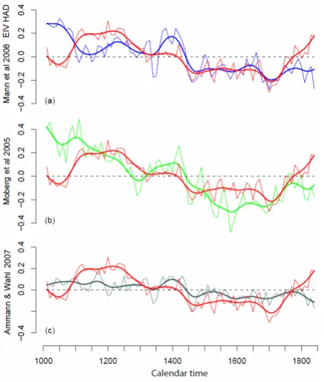
Fig. 2. Comparisons between thee recent reconstructions of the Northern Hemisphere surface temperature with SGI (red lines), on the 1000–1850 AD period. The upper panel (a) shows the recon-struction provided by (Mann et al., 2008) (blue lines), using both land and ocean data with the EIV method. On panel (b) the green lines correspond to the reconstruction of (Moberg et al., 2005), and the lower panel (c) shows the reconstruction of (Ammann and Wahl, 2007) (blue grey lines). The thin lines are the 10yr-running mean time series, sampled every ten years, and the thick lines are the cubic spline equivalent in number of degrees of freedom to a 50yr-running mean. The anomalies are calculated relative to the 1000–1850 pe-riod.
(SW2010 hereafter) chosen here because they used similar solar and GHGs forcings as used in the present study. They also take into account volcanic forcing during the last mil-lennium, with a TSI damping to represent the direct radia-tive impact of the volcanoes in IPCC AR4 simulations, or with a reconstruction of the optical thickness of the volcanic aerosols in SW2010. This allows a comparison of the NH temperature secular variability between SGI and similar nu-merical exercises available using a volcanic forcing.
as analogues of the MCA for the warm period and the LIA for the cold period.
For a quantitative evaluation of the NH temperature vari-ability in SGI we compared our simulation with three recent Northern Hemisphere temperature reconstructions (Fig. 2), provided by (Ammann and Wahl, 2007) (AW07 hereafter), (Moberg et al., 2005) (Mob05 hereafter) and the tempera-ture reconstruction obtained with the Error In Variables re-construction method, calibrated on land and ocean data by (Mann et al., 2008) (M08 hereafter). The reconstructions show different amplitudes of temperature secular evolution, and reflect the important uncertainties linked to the proxy and the reconstruction method used. We can infer consistent in-formation from those datasets only when a common pattern is identified. We smoothed both SGI NH temperature and temperature reconstructions time series with a 10-year run-ning mean and sampled every 10 years to respect the number of degrees of freedom. We also computed an estimate of the lower frequency evolution with a cubic spline function (Green and Silverman, 1994) with seventeen degrees of free-dom, corresponding to a∼50-year running mean.
The variance of the ten-year smoothed SGI time series between 1000 and 1850 AD is 0.037◦C2. It lies between the variance of Mob05 (0.05◦C2)and M08 (0.024◦C2)and supports the realistic amplitude of the variability in the SGI simulation. The correlation coefficients with Mob05 and M08 are 0.59 and 0.4 (p-value<10−5) respectively, and 0.18 with AW07 (p-value<0.09). The correlation coeffi-cients between the reconstructions range from 0.67 to 0.8 (p-value<2.10−16). The SGI simulation shows less agreement with the temperature reconstructions than the reconstructions between them.
The temperature maximum occurs around 1200 AD in SGI, whereas it appears around 1000 AD in the reconstruc-tions overlap. The amplitude of the temperature variability in AW07 is too weak to robustly identify a centennial warm period during the MCA. During the first two centuries of the millennium, SGI presents a trough with a minimum around 1075 AD. This behaviour is also observed in the IPCC sim-ulations forced by similar TSI variability, even when repre-senting the effect of volcanic aerosols. During the same pe-riod Mob05 and M08 show a maximum around 1000 AD and a continuous decrease of the temperature until 1200 AD. This evolution is supported by the reconstructions overlap with good confidence.
Between 1200 and 1700 AD, the temperature in SGI de-creases as in M08 and Mob05. The NH temperature of SGI shows common extremes with the reconstructions around 1400 and 1450 AD and with M08 and Mob05 around 1700 AD. The cold period identified as the LIA in SGI begins around 1400 AD as well as in the reconstructions, with a minimum around 1700 AD in SGI and M08. In Mob05 the temperature evolution shows a similar shape as SGI between 1400 and 1850 AD, but the minimum occurs around 1500 AD in Mob05. In AW07 the coldest period occurs after 1850
AD (not shown), two centuries later than in SGI, M08 and Mob05. The warming simulated by the model between 1750 and 1850 AD is stronger than in the reconstructions, poten-tially because of the missing impact of volcanoes. After 1400 AD, the NH temperature evolution in SGI is in better general agreement with the temperature reconstructions than before 1200 AD.
The industrial part of SGI warms strongly compared to the reconstructions and the IPCC and SW2010 simulations be-cause of the missing volcanoes. We confirmed this hypoth-esis by running an additional simulation covering the 1850-2000 AD period (VHIST), starting from SGI in 1850 AD, with the volcanic forcing (not shown) used in the ENSEM-BLE project (Royer et al., 2009). The resulting temperature evolution (Fig. 1c) is in better agreement with both recon-structions and IPCC simulations.
3.2 Forcing signature on NH temperature
For a critical assessment of the NH temperature variability in the preindustrial part of SGI we quantified the role of solar, CO2and orbital forcings on the NH temperature variability in the simulation. It implies evaluating the temperature vari-ability due to internal processes and the part attributed to the forced variability. We hence used a statistical method based on a linear decomposition of the temperature anomalies dT as the sum of the first order contributions, or signatures, of external forcingsEi and an associated residual noiseε:
dT=X i
∂T
∂Ei
dEi+ε.
Following this decomposition we propose the follow-ing statistical linear model to describe the NH temperature anomalies in the simulation SGI (Fig. 3):
T0(t )=C1×TSI0(t )+C2× [CO2]0(t)+ε(t),
witht is the time index, T0, TSI’ and [CO2]0 the anoma-lies relative to the 1000–1850 period NH temperature, TSI and CO2concentrations respectively,C1=(∂T0/∂TSI0)and C2=(∂T0/∂[CO2]0)the first order sensitivity of the model to TSI and CO2respectively, andε(t) the residual noise. The first step is to test the null hypothesis that only one forcing with an associated residual noise can explain the NH temper-ature variability. We estimatedC1andC2with both univari-ate (C1UVandC2UV) and bivariate (C1BVandC2BV) linear regressions, following the nested regression models: T0(t )=C1UV×TSI0(t )+ε1(t ), (1) T0(t )=C2UV× [CO2]0(t)+ε2(t) (2) T0(t )=C1BV×TSI0(t )+C2BV× [CO2]0(t)+ε3(t) (3) We calculated the signatures associated with TSI (S(1TSI)= C1UV×TSI’(t)), CO2 (S2(CO2)=C2UV[CO2]0(t) ), the total
450 J. Servonnat et al.: Influence of solar variability, CO2and orbital forcing
Table 1. Variances of the Northern Hemisphere temperature (T) in SGI and the signatures of solar (S1) and CO2(S2) forcing estimated on the whole period, the first part (1000–1425 AD) and the second part of the millennium (1425–1850 AD). The indices UV and BV denote the methods to estimate the coefficients, i.e. univariate and bivariate regressions, respectively.
1000–1850 1000–1425 1425–1850
(MCA) (LIA)
var(T0)×10−2 1.9 1 1.2
var(SUV1 )×10−2 1.1 0.78 0.34
var(SUV2 )×10−2 0.7 0.06 0.32
var(SBV1 )×10−2 0.8 0.85 0.49
var(SBV2 )×10−2 0.4 0.005 0.45
var(Stot)×10−2 1.5 0.9 0.77
signature (Stot=S3(TSI)+S(CO2)
3 ), with S3(TSI)=C1BV× TSI0(t ) and S3(CO2)=C2BV× [CO
2] and their correlation coefficients with the temperature anomaliesT0 to evaluate which model performs the best in reproducing the NH tem-perature variability of SGI. The variances of the signatures are reported in Table 2. We calculated the linear regression coefficients between the residuals associated with the uni-variate models shown by Eq. (1) and Eq. (2) and the CO2 and TSI time series respectively to verify if a significant sig-nal corresponding to a neglected forcing is detected. Fisig-nally we estimated the slope of the residualsε3to detect a possible trend in temperature associated to changes in insolation due to orbital forcing. We applied those analyses over the whole 1000–1850 period, the first part of the millennium enclos-ing the MCA (between 1000 and 1425 AD) and the second part assumed as the LIA (1425–1850 AD). The results are reported in Table 1.
On the 1000–1850 period, the termsS1(TSI)andS(CO2)
2
ex-plain 59% and 36% of the total variance of T0. The cor-relation coefficient ofS(1TSI) withT0 is 0.76 while between S(CO2)
2 andT
0the value is 0.6. The residualsε1andε2are
significantly (99.5% level) correlated to [CO2]0and TSI’ re-spectively and the corresponding regression coefficients lie between the confidence intervals of the coefficientsCBV1 and C2BV.
It shows that only one forcing is not enough to explain the total forced variability in the simulation. The null hypothesis held by Eq. (1) and Eq. (2) is thus rejected when considering the full preindustrial period. The variance explained by the term in Eq. (3) represent 78% of the total variance ofT0, with a correlation r=0.88 (p-value<2.10−16). The slope of the residualsε3is−0.08◦C/1000 yr and is poorly significant
(p-Table 2. Sensitivity coefficients to solar (C1) and CO2 (C2) es-timated on the Northern Hemisphere temperature in SGI, on the whole preindustrial period, the MCA and the LIA. The indices UV and BV denote the methods to estimate the coefficients, i.e. univari-ate and bivariunivari-ate regressions, respectively.
1000–1850 1000–1425 1425–1850 (MCA) (LIA)
C1UV(◦C/Wm−2) 0.117±0.011 0.13±0.01 0.07±0.02 C2UV(◦C/ppm) 0.029±0.004 0.04±0.01 0.016±0.004 C1BV(◦C/Wm−2) 0.10±0.009 0.13±0.02 0.08±0.01 C2BV(◦C/ppm) 0.022±0.003 0.005±0.008 0.019±0.003
value∼0.01), confirming that orbital forcing can be neglected at hemispherical scale in annual average. The first order sensitivity of the NH temperature in the model to TSI vari-ability and CO2for the total preindustrial period estimated with bivariate linear regression isC1BV=0.10◦C/W/m2and C2BV=0.0022◦C/ppm, respectively. The separated signa-tures of the bivariate modelS3(TSI),S(CO2)
3 and the residuals ε3explain respectively 45, 20 and 22% of the total variance. The covariance term due to both solar and CO2forcings (2× cov(S3(TSI), (S(CO2)
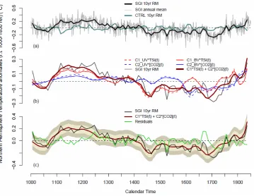
3 ) is equivalent to 13% of the total variance ofT0. Theε3residuals and the NH temperature anomalies of the CTRL simulation have similar variance and covariance. The bivariate model (3) is in very good visual agreement with SGI (Fig. 3), which gives good confidence on the ro-bustness of the decomposition with the statistical model held by Eq. (3). We infer that on the whole 1000–1850 AD pe-riod the response of the model to the forcings dominates the NH temperature signal in the SGI simulation, and that the TSI variability has a stronger influence than the variations in CO2concentration. This model also estimates that 13% of the total variance ofT0is due to the joint contribution of TSI and CO2.
We repeated the analysis on the first part of the millen-nium covering the MCA. The estimates ofC1BVandC2BVon the 1000–1425 AD time interval give a significantly greater value forC1BV (0.13◦C/Wm−2), and C2BVis not significant (0.005◦C/ppm, pvalue>50). The correlation between TSI’ andT0is 0.86, and 0.6 between [CO2]’ andT0. The variance of the signatureS(1TSI)corresponds to 79% of total variance, versus 88% for the total signatureStot. The variance of the signature of CO2is weak in front of the variance of the sig-nature of TSI, indicating that the null hypothesis represented by Eq. (1) is verified. This analysis clearly shows that solar forcing dominates the NH temperature variability in the first part of the simulation.
During the second part of the millennium (LIA), the vari-ance of the signatures of the univariate models S1(TSI) and S(CO2)
29
1
Figure 3: (a) surface temperature anomalies relative to 1000-1850 AD reference period averaged over the
2
Northern Hemisphere in SGI, on annual mean (grey line). The thick black line is the ten-year running mean
3
applied on the annual averages, sampled every ten years to keep the number of degrees of freedom. The same
4
treatment is done on the CTRL simulation, drawn on grey blue. (b) Fingerprints of solar (red lines) and CO2
5
(blue lines) forcings, estimated with univariate (dashed lines) and bivariate linear regressions and anomalies of
6
TSI and CO2 concentrations relative to the 1000-1850 AD period. The fingerprint of both solar and CO2 forcings
7
together is represented by the dark red line. The black thin line shows the 10yr-running mean of the NH
8
temperature of SGI presented on panel (a). (c) Fingerprint of both solar and CO2 forcings together (dark red
9
line). The residuals corresponding to SGI minus total forced fingerprint are represented by the green line. The
10
light shaded area shows the interval corresponding to ±1 standard deviation (SD) of the residuals, and the dark
11
shaded area depicts the ±2SD of the residuals. The black line plotted over is the ten-year NH temperature of SGI
12
presented on panel (a).
13
Fig. 3. (a) Surface temperature anomalies relative to 1000–1850 AD reference period averaged over the Northern Hemisphere in SGI, on annual mean (grey line). The thick black line is the ten-year running mean applied on the annual averages, sampled every ten years to keep the number of degrees of freedom. The same treatment is done on the CTRL simulation, drawn on grey blue. (b) Fingerprints of solar (red lines) and CO2blue lines) forcings, estimated with univariate (dashed lines) and bivariate linear regressions and anomalies of TSI and CO2 concentrations relative to the 1000–1850 AD period. The fingerprint of both solar and CO2forcings together is represented by the dark red line. The black thin line shows the 10 yr-running mean of the NH temperature of SGI presented on panel (a). (c) Fingerprint of both solar and CO2forcings together (dark red line). The residuals corresponding to SGI minus total forced fingerprint are represented by the green line. The light shaded area shows the interval corresponding to 1 standard deviation (SD) of the residuals, and the dark shaded area depicts the±2SD of the residuals. The black line plotted over is the ten-year NH temperature of SGI presented on panel (a).
T0 respectively. BothS1(TSI) andS(CO2)
2 are less correlated toT0 than on the whole preindustrial period (0.52 for TSI and 0.49 for CO2)because they vary in opposite direction between 1450 and 1700 AD and are significantly detected during the LIA. The solar forcing signal is detected with a significantC1UVcoefficient inε2as well as the CO2signal in ε1. The null hypothesis of either model (1) or model (2) is rejected. The estimates ofCBV1 andC2BVgiveS3(TSI),S(CO2)
3 andStot terms that correspond to 39, 36 and 61% of total variance, with a negative covariance term equivalent to 13% ofT0total variance. The correlation between the total finger-printStot andT0 is 0.78. This confirms that solar and CO2 together explain the NH temperature variability in SGI dur-ing the LIA better than one forcdur-ing at a time. The variance of the residualsε3corresponds to 38% of the total variance of T0. The decomposition ofT0with the bivariate model (Eq. (3)) between 1425 and 1850 AD attributes a lower part of the temperature variability to the external forcings than on the whole preindustrial period or the first part of the millennium.
To complete this analysis, we have computed the bivariate linear regression betweenT0and both forcings taking into ac-count a lag to catch a possible memory of the climate system. The coefficients obtained (not shown) show maximum values when the forcings precede the temperature by one to three decades, highlighting a memory effect likely attributable to the heat capacity of the oceans. However, the maximum co-efficients lie in the confidence interval of the first estimate of C1BVandC2BV. Taking into account a memory parameter in the statistical model held by Eq. (3) would not change dra-matically the part of the total variance attributable to solar or GHG forcing.
The NH temperature in the SGI simulation shows a vari-ance close to NH temperature reconstructions and IPCC sim-ulations achieved with comparable secular forcings. The re-sponse of the model to the forcings on the whole preindus-trial period is mainly linear. The LIA is driven at first or-der by both TSI and CO2 and the minimum around 1700 AD is similar to the minimum identified in reconstructions. The evolution of the temperature during the first part of the
452 J. Servonnat et al.: Influence of solar variability, CO2and orbital forcing
30 1
Figure 4: second to fifth step of the algorithm cutting the surface of the Earth in individual areas. N is the 2
number of areas delimited by the bluetraight lines, and s the step in the algorithm. The surface temperature time 3
series are averaged over all the individual areas to calculate the SNR. 4
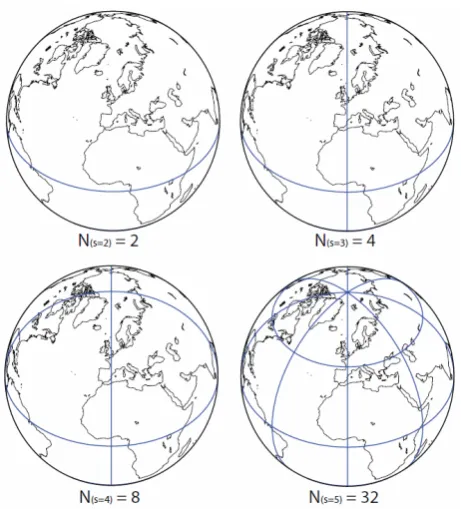
Fig. 4. Second to fifth step of the algorithm cutting the surface of the Earth in individual areas.Nis the number of areas delimited by the bluetraight lines, andsthe step in the algorithm. The surface temperature time series are averaged over all the individual areas to calculate the SNR.
millennium, at∼80% linearly driven by solar forcing in SGI, appears to be different from the reconstructions, with the warmer period occurring two centuries later than in most of the records.
4 Multiscale signature of the forced variability
We have seen in the previous section that the Northern Hemi-sphere temperature in the SGI simulation is driven at 78% by the model response to the forcings, mostly represented by TSI variability. We now check whether this can be trans-posed to small geographical scales. The relative importance of forced and internal variability in a temperature signal de-pends on the radiative perturbation imposed as well as the in-fluence of internal processes on the considered area. Ocean-atmosphere dynamics such as the El Ni˜no Southern Oscilla-tion (ENSO) in the Pacific Ocean or the North Atlantic Os-cillation (NAO) over the North Atlantic sector are sources of important temperature variations that can be detected at the hemispherical or continental scale, while local processes involving meteorological phenomenon mix the signature of global forcings with a noise inherent to the climate system. All those internal processes are more or less independent, and their influence on the signal tends to vanish when aver-aging the temperature over large extents. In this section we
31 1
Figure 5:Signal-Noise Ratio (SNR) calculated as a function of the spatial scale with the ratio of variance
2
between the temperature in SGI and the CTRL described in Sec. 4. On the upper x-axis is the extent of the
3
surface associated with the SNR. The lower x-axis gives references of geographic dimensions. The black, blue
4
and red lines represent the SNR calculated with temperature time series smoothed with a 51, 31 and
11yr-5
running mean respectively. The black, blue and red dashed lines represent the 99th
quantile of the Fisher
6
distribution with 17, 28 and 85 degrees of freedom (dof) equivalent to the number of dof of a 850-year long time
7
series smoothed with 51, 31 and 11yr-running mean respectively.
8
Fig. 5. Signal-Noise Ratio (SNR) calculated as a function of the spatial scale with the ratio of variance between the temperature in SGI and the CTRL described in Sect. 4. On the upper x-axis is the extent of the surface associated with the SNR. The lower x-axis gives references of geographic dimensions. The black, blue and red lines represent the SNR calculated with temperature time series smoothed with a 51, 31 and 11 yr running mean respectively. The black, blue and red dashed lines represent the 99th quantile of the Fisher distribution with 17, 28 and 85 degrees of freedom (dof) equivalent to the number of dof of a 850-year long time series smoothed with 51, 31 and 11 yr-running mean, respectively.
assess the response of the IPSLCM4 climate model to solar, GHG and orbital forcings at spatial scales ranging from the globe to the individual cells of the model grid.
The next analysis estimates the characteristic spatial scale under which the temperature variance of our forced simula-tion SGI is comparable to the corresponding variance of the CTRL run, i.e. the model internal variability. We propose an estimate of the ratio between the variance of the temperature in SGI and in the CTRL as a function of the spatial scale con-sidered, based on the additivity of the variance. We split the surface of the globe inN areas, and compute the tempera-ture time series averaged over thoseNareas for both the SGI and the CTRL simulations. We then estimate a signal-noise ratio (SNR hereafter) defined as the ratio between the sum of the variances of theN temperature time series in the SGI simulation and the sum of the variances of the corresponding time series in the CTRL, weighted by the root mean square of their associated areas, for thesstep needed to cut the globe in individual grid point with the cutting algorithm:
SNR(s)= PN
i (s)var(TSGI,i)×αi PN
i (s)var(TCTRL,i)×αi
(4)
whereαi is the surface of the ith area on which the
temper-ature time series of SGITSGI,i is averaged, and var(TSGI,i)
32
1
Figure 6: first order sensitivity of the temperature in SGI to TSI variability estimated by C1BV expressed in
2
°C/Wm-2 (a,b,c,), to CO2 by C2BV expressed in °C/ppm (d,e,f), and slope of the ε3 residuals corresponding to C3
3
expressed in °C/1000yr (g,h,i). Those coefficients are calculated for annual (a,d,g), summer (b,e,h,
June-July-4
August) and winter (c,f,i, December-January-February) averages. The white areas represent the grid points
5
where the coefficients are not significant at 99.5% (Student t test).
6
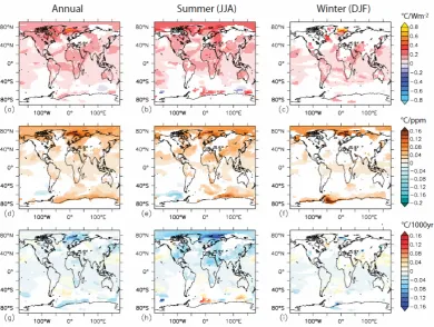
Fig. 6. First order sensitivity of the temperature in SGI to TSI variability estimated byCBV1 expressed in◦C/Wm−2(a, b, c), to CO2by CBV2 expressed in◦C/ppm (d, e, f), and slope of theε3residuals corresponding toC3expressed in◦C/1000 yr (g, h, i). Those coefficients are calculated for annual (a, d, g), summer (b, e, h, June-July- August) and winter (c, f, i, December-January-February) averages. The white areas represent the grid points where the coefficients are not significant at 99.5% (Studentttest).
considered as significantly different from the variance of the denominator when the SNR is greater than the 99th quantile of the Fisher distribution with a number of degrees of free-dom equivalents to the number of degrees of freefree-dom (Von Storch and Zwiers, 2001) of the time series. The cutting al-gorithm is illustrated in Fig. 4. The first estimate of the SNR is done with the global meanN(s=1)=1. We then split the
Earth by the equator for the second estimateN(s=2)=2. The
hemispheres are then separated in two parts for the third step N(s=3)=4. The following steps consist in splitting every
area of the previous step by the middle of its sides to obtain the next four zones (N(s=i)=4×N(s=i−1)), until reaching
the grid point. The spatial scale of a given step is calculated by computing the average of the extents of all the sectors. We estimate the SNR with time series smoothed with eleven-year, thirty one-year and fifty one year running mean to test the sensitivity of the ratio to the frequency of the variabil-ity considered. The results are shown in Fig. 5. The SNR is maximum at global scale and minimum at the grid point scale. It is high at the hemispherical scale as inferred from previous section. It shows a continuous decrease and reaches the significance threshold between 3 and 7.106km2, for all
the smoothing applied on the time series. The slopes of the SNR curves are too low around the significance level to deter-mine the dependence between the characteristic spatial scale and the frequency of the variability (smoothing) considered. For a given spatial scale, the SNR is higher with the lower frequency time series because of the frequency of the forc-ings imposed. The characteristic spatial scale of detectabil-ity of the forced signal is 5.106km2, between the extent of Australia and Europe.
This first approach invites us to go deeper in the details of the sensitivity of the model in SGI around the Globe. The next step is to assess the local sensitivity of the model to solar, GHGs and orbital forcings. For every model grid point, we apply the statistical decomposition (3) used to describe the NH temperature in the previous section, and add a term corresponding to the influence of orbital forcing:
T0(t )=C1×TSI0(t )+C2× [CO2]0(t)+C3× +t+ε4 (5) with C3the slope of theε3residuals, attributed to the linear changes in insolation, andε4 the residual noise of Eq. (5). The decomposition is done on annual, winter (December-January-February, DJF hereafter) and summer mean (June-July-August, JJA hereafter) on series smoothed with an
454 J. Servonnat et al.: Influence of solar variability, CO2and orbital forcing
1
Figure 7: Percentage of temperature variance explained at first order by the terms in equation (4) corresponding
2
to the fingerprints of solar (d, e, f), CO2 (g, h, i), and orbital (j, k, l) forcings, and of all the forcings together (m,
3
n, o). The white areas depicts the grid points where the fingerprints explain less than 5% of the total variance of
4
the temperature at the given grid points, or where the regression coefficients shown on Figure 5 are not
5
significant at 99.5%. The upper panels (a, b, c) show the temperature variance of the ten-year smoothed time
6
series used in this study. All those diagnostics are done on annual (a, d, g, j, m), summer (b, e, h, k, n) and winter
7
averages (c, f, i, l, o).
8
Fig. 7. Percentage of temperature variance explained at first order by the terms in Eq. (4) corresponding to the fingerprints of solar (d, e, f), CO2(g, h, i), and orbital (j, k, l) forcings, and of all the forcings together (m, n, o). The white areas depicts the grid points where the fingerprints explain less than 5% of the total variance of the temperature at the given grid points, or where the regression coefficients shown on Fig. 5 are not significant at 99.5%. The upper panels (a, b, c) show the temperature variance of the ten-year smoothed time series used in this study. All those diagnostics are done on annual (a, d, g, j, m), summer (b, e, h, k, n) and winter averages (c, f, i, l, o).
eleven-year running mean, sampled every ten years, so that the analysis focus on decadal and longer variability. The re-gression coefficients (Fig. 6) measure the first order sensitiv-ity of the temperature to the forcings (C1is in◦C/Wm−2and C2is in◦C/ppm).
Additionally we evaluated the percentage of the total vari-ance of temperature at every grid point associated to the sig-natures of the forcings in Eq. (4) (Fig. 7), as done in Sect. 3 for the NH temperature. The white areas in Fig. (6) repre-sent the grid points where the regression coefficients are not
significant and the white areas in Fig. (7) show where the variance of the signatures explain less than 5% of the total variance at the grid point. This means that the temperature variability is dominated by internal processes or that the tem-perature variance is mainly explained by another forcing.
34 1
Figure 8 : comparison between the Arctic summer temperature reconstruction provided by (Kaufman et al., 2
2009) (grey and black lines) and SGI. The orange and red lines show the summer mean in SGI. The blue lines 3
show the residuals calculated as the summer temperature time series in SGI, minus the signatures of TSI and 4
CO2 (equivalent to the ε3 residuals in equation (3)). The grey, orange and light blue thin lines represent the ten-5
year smoothed time series of (Kaufman et al., 2009), SGI summer mean and SGI summer residuals respectively. 6
The thick black, red and blue lines show the linear regressions associated with the summer temperature time 7
series of (Kaufman et al., 2009), SGI summer mean and SGI summer residuals respectively. 8
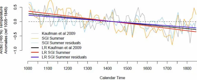
Fig. 8. Comparison between the Arctic summer temperature reconstruction provided by (Kaufman et al., 2009) (grey and black lines) and SGI. The orange and red lines show the summer mean in SGI. The blue lines show the residuals calculated as the summer temperature time series in SGI, minus the signatures of TSI and CO2(equivalent to theε3residuals in Eq. 3). The grey, orange and light blue thin lines represent the ten-year smoothed time series of (Kaufman et al., 2009), SGI summer mean and SGI summer residuals, respectively. The thick black, red and blue lines show the linear regressions associated with the summer temperature time series of (Kaufman et al., 2009), SGI summer mean and SGI summer residuals, respectively.
explained by the latitude-months forcing patterns associated with variations in TSI and CO2, as illustrated in (Govin-dasamy et al., 2003) and (Dufresne et al., 2005).
The sensitivity to TSI (C1) is important in the tropics (∼0.2◦C/Wm−2)and of comparable amplitude on annual, summer and winter averages likely because the solar radia-tive forcing is almost constant with the seasons in this region. In the Northern high latitudes, the model sensitivity to solar forcing shows strong differences between summer and win-ter, reflecting the seasonal dependence of solar forcing with the latitude.
The sensitivity to CO2shows less contrasted patterns be-tween summer and winter in high latitudes than sensitivity to TSI variations. This is consistent with the weaker seasonal cycle of the CO2radiative forcing in the Arctic region.
In the Southern Hemisphere the ocean-atmosphere-sea-ice dynamics around Antarctica generate important decadal to multi-decadal variability and the significant coefficients are restricted to small areas.
The slope C3 shows the higher values in the Northern Hemisphere during summer and the highest values in the Arctic. On annual and winter mean theC3 values do not show any latitudinal coherence, denoting that those trends are probably not linked to orbital forcing.
The temperature variance in SGI (Fig. 7) is the strongest in the high latitudes as well as the sensitivity to TSI, CO2 and orbital forcing. The amount of variance explained by the signature of solar forcing in SGI is not strictly following the values of sensitivity to TSI variability. The temperature vari-ance in the equatorial band is particularly affected by solar forcing because solar irradiance is high around the equator. The signature of TSI explains more than 50% of the tem-perature variance in the Western Pacific Ocean (Warm Pool), the Indian Ocean and the Equatorial Atlantic Ocean. It has
lower impact in the Arctic despite higher sensitivity values. It explains more than 10% of the temperature variance over most of the continents on annual average, in North and South America, Africa, and Southern Asia. It is weakly significant over Europe on annual average and winter, and the variance of its signature can reach 25% of temperature variance in summer. At mid-latitudes, the variance explained by solar forcing in winter and summer follows the associated sensi-tivity patterns.
The signature pattern of CO2 follows the C2 sensitivity pattern. It reaches∼25% of the temperature variance in the Polar Regions and Europe on annual averages and∼25% of the temperature variance over Eastern Asia on summer aver-ages. It shows a weak signature in the tropical area (∼10% of the temperature variance).
The higher values of the variance of the signature of or-bital forcing follow the strong values of theC3 coefficient, and occur during summer in North Africa and in the Arctic region. This behaviour reflects the latitudes where the orbital forcing has the biggest amplitude since the changes in the orbital parameters modulate essentially the solar input in the Polar regions during their respective summer.
We have compared the temperature of the SGI simula-tion to the summer temperature reconstrucsimula-tion over Arctic (>65◦N) of Kaufman et al. (2009) (K09 hereafter). They
found that their temperature record was following a linear decrease that they attributed to changes in insolation due to the precession of the equinoxes during the last two millen-nia. We calculated the annual and summer temperature above 65◦N in SGI (Y65 and S65), and applied the same smooth-ing as in K09. We also removed the linear contributions of TSI and CO2 from the two time series calculated in SGI to focus on the signal due to orbital forcingC3×t (Y65ε3 and S65ε3. Finally we estimated the slope of each time
456 J. Servonnat et al.: Influence of solar variability, CO2and orbital forcing
35 1
Figure 9: Percentage of Earth surface (on x-axis) where the variances of the signatures of the forcings used in 2
SGI explain at least the percentage of temperature variance represented on y-axis. This diagnostic is represented 3
for solar (red line), CO2 (blue line) and orbital (orange line) forcing and for all the forcings together (black line).
4
The horizontal dashed lines underline 25 and 50% of temperature variance. 5
6
Fig. 9. Percentage of Earth surface (on x-axis) where the variances of the signatures of the forcings used in SGI explain at least the per-centage of temperature variance represented on y-axis. This diag-nostic is represented for solar (red line), CO2(blue line) and orbital (orange line) forcing and for all the forcings together (black line). The horizontal dashed lines underline 25 and 50% of temperature variance.
series, including the temperature reconstruction of K09 be-tween 1005 and 1845 AD. The time series are represented in Fig. 8. The slope estimated in K09 (−0.65±0.1◦C/1000 yr)
lies between the slope of Y65 (−0.5±0.12◦C/1000 yr) and S65 (−0.85±0.12◦C/1000 yr) time series. With the time se-ries Y65ε3andS65ε3, we found no significant slope for the former (−0.2±0.1◦C/1000 yr) and (−0.52±0.9◦C/1000 yr) for the latter. This last result is close to the slope found with K09 and underlines the important impact of orbital forcing at high latitudes in summer during the last millennium. It is however negligible on annual and winter average in SGI as seen in Fig. 7.
All the forcings together explain up to∼70% of the tem-perature variance on annual and summer averages over the equatorial area. Half of the temperature signal in the Arctic is explained by the forced variability. The total forced signal is found almost everywhere over land and explains in major-ity between 20 and 50% of temperature variance.
We synthesize the global information of Fig. 7 by comput-ing the percentage of Earth’s surface where the signature of
the forcings (Eq. 4) represents more than a given percentage of temperature variance (Fig. 9). On annual average, there is only∼30% of the surface of the Earth where at least 50% of the temperature variance is explained at first order by all the forcings used in SGI. Solar forcing represents the biggest part of the forced signal on the widest extent compared to the other forcings, on annual, summer and winter average. On summer averages, orbital forcing explains more than 10% of temperature variance over 10% of the surface of the Earth. The signature of CO2represents more than 5% of the total variance of temperature on only 20% of the surface of the Earth, on both annual and summer averages. We detect the total forced signal (>10% of the total variance) on annual and summer average on∼70% of the globe. On annual aver-age,∼10% of the surface of the Earth is largely dominated by the total forced signal (>80% of the total temperature vari-ance), in a similar proportion than the NH temperature of SGI.
We found that the characteristic spatial scale to detect a forced temperature signal significantly different from inter-nal variability is∼5.106km2. The sensitivity to TSI and CO2 is the highest in the polar regions, especially in the Arctic. The solar forcing explains ∼50% of the temperature vari-ance in the tropics. Its signature is dominant compared to CO2 in both spatial extent and amplitude. Orbital forcing has a significant signature in the Arctic summer temperature and supports the conclusion of K09. Half of the temperature variance is explained at first order by forced variability on ∼30% of the Earth’s surface.
5 Discussion and conclusion
We have performed two millennium-long simulations with the IPSLCM4 climate model to evaluate the impact of To-tal Solar Irradiance variability, CO2 and orbital forcing on temperature during the last millennium. The SGI (Solar, Greenhouse gas and Insolation) simulation reproduces well the temperature evolution during the last millennium around the LIA. The amplitude of the NH temperature secular vari-ability is in agreement with both temperature reconstructions and previous simulations (IPCC AR4 and SW2010) using similar solar and CO2 forcings but taking into account the impact of the volcanoes. We found an important difference between the reconstructions and SGI between 1000 and 1200 AD, which also appears in the IPCC AR4 simulations.
On the second part of the simulation (after 1425 AD), CO2 and TSI explained equivalent proportion of NH temperature variance. This result shows a similar implication of CO2on temperature variations during the LIA as found by (Hegerl et al., 2007).
The mismatch during the beginning of the millennium is potentially due to uncertainties on the initial state of the ocean and uncertainties in the reconstructions. Nevertheless, we can have a critical view on the experimental setup. The mismatch implies that the secular variability of the NH tem-perature reconstructions during the MCA is not explained by the response of the model, mainly linear, to the TSI recon-struction. The use of a TSI reconstruction presenting lower amplitude will decrease the difference between reconstruc-tions and simulareconstruc-tions during this period, but will also weaken the temperature decrease between the MCA and the LIA. Lower amplitude of the secular temperature variability would be in better agreement with NH temperature reconstructions as AW07.
The IPCC AR4 and SW2010 simulations taking into ac-count the impact of the volcanoes show secular NH temper-ature evolution very similar to SGI. Volcanic forcing seems to have a weak impact on secular NH temperature variability compared to the solar forcing used in SGI and IPCC AR4 simulations shown, i.e. with a TSI mean value during the Maunder Minimum 0.25% lower than modern value. With lower amplitude of TSI variability, the influence of cumu-lative eruptions on secular temperature variability would be different (Ammann et al., 2007; Gao et al., 2009; Hegerl et al., 2007).
We evaluated the significance of a variance ratio between the SGI simulation and the CTRL simulation with an esti-mate of a signal-noise ratio dependant on the spatial scale considered. We found that the temperature signal of the forced simulation SGI is significantly (99% level) different from internal variability for area wider than ∼5.106km2, i.e. an extent equivalent to Europe. This characteristic spa-tial scale is suitable for the TSI, CO2 and orbital forcings used in SGI and for this spatial resolution of IPSLCM4. The solar forcing had the most extended spatial signature on local temperature, and explained the most important part of tem-perature variance. Polar Regions are the most sensitive areas to the three forcings. The temperature variance in the equa-torial band is the most affected zone by forced variability, essentially because of solar forcing. Orbital forcing is de-tected over 65◦N in summer, which support the conclusions
of (Kaufman et al., 2009). We found that the signature of the total forced variability was greater than 10% almost ev-erywhere over land, but the total forced variability represent at least half of the temperature signal on only∼30% of the surface of the globe.
The study of the SNR and local signatures of the forcings suggests that individual temperature reconstructions taken from random location around the globe are weakly affected by the linear response of the temperature to the forcings. It is
necessary to reconstruct temperature during the last millen-nium over sufficiently large spatial extent to capture a tem-perature signal significantly affected by the forcings. The proxies used to reconstruct the temperature like tree rings, pollens or lake sediments are sensitive to the summer sea-son when the temperature signal is the most affected by the forcings in SGI. This study highlights areas where the tem-perature variance is dominated by the forced signal. It will be extended to other climatic simulations on the last millen-nium taking into account a reconstruction of the optical depth of volcanic aerosols (Gao et al., 2009) with IPSLCM4 and a simulation performed with another coupled GCM (SW2010). A next step will consist of using a coupled GCM with a finer vertical resolution in the stratosphere and interactive ozone chemistry (Shindell et al., 2001; Meehl et al., 2009) allowing a dynamical response of the model to solar forcing.
Our study shows that the role of solar variability on sec-ular temperature evolution during the last millennium is still not fully understood, especially during the MCA. There is a need for more complete spatial coverage of proxy records, focused on strategic locations where the signal of external forcing should be important compared to internal variability.
Acknowledgements. This work was supported by the ANR ESCARSEL project. The authors would also like to credit the contributors of the R project.
Edited by: M. Claussen
The publication of this article is financed by CNRS-INSU.
References
Ammann, C., Joos, F., Schimel, D., Otto-Bliesner, B., and Tomas, R.: Solar influence on climate during the past millen-nium: Results from transient simulations with the ncar climate system model, Proc. Nat. Acad. Sci. USA, 104, 3713–3718, doi:10.1073/pnas.0605064103, 2007.
Ammann, C. and Wahl, E.: The importance of the geophysical context in statistical evaluations of climate reconstruction pro-cedures, Climatic Change, 85, 71–88, doi:10.1007/s10584-007-9276-x, 2007.
Bard, E., Raisbeck, G., Yiou, F., and Jouzel, J.: Solar irradiance during the last 1200 years based on cosmogenic nuclides, Tellus B, 52, 985–992, 2000.
Bauer, E., Claussen, M., Brovkin, V., and Huenerbein, A.: Assess-ing climate forcAssess-ings of the earth system for the past millennium, Geophys. Res. Lett., 30, doi:10.1029/2002gl016639, 2003.
458 J. Servonnat et al.: Influence of solar variability, CO2and orbital forcing
Bertrand, C., Loutre, M. F., Crucifix, M., and Berger, A.: Climate of the last millennium: A sensitivity study, Tellus A, 54, 221–244, doi:10.1034/j.1600-0870.2002.00287.x 2002.
Bjune, A., Birks, H. J. B., and Seppa, H.: Holocene vegetation and climate history on a continental-oceanic transect in northern fennoscandia based on pollen and plant macrofossils, Boreas, 33, 211–223, doi:10.1080/03009480410001244, 2004.
Boucher, O. and Pham, M.: History of sulfate aerosol radiative forc-ings, Geophys. Res. Lett., 29, doi:10.1029/2001gl014048, 2002. Bradley, R., Hughes, M., and Diaz, H.: Climate in medieval time,
Science, 302, 404–405, doi:10.1126/science.1090372, 2003. Brazdil, R., Pfister, C., Wanner, H., Von Storch, H., and
Luter-bacher, J.: Historical climatology in europe – the state of the art, Clim. Change, 70, 363–430, 2005.
Briffa, K. R., Osborn, T. J., and Schweingruber, F. H.: Large-scale temperature inferences from tree rings: A review, Global Planet. Change, 40, 11–26, doi:10.1016/S0921-8181(03)00095-X, 2004.
Cook, E., Palmer, J., and D’Arrigo, R.: Evidence for a ’medieval warm period’ in a 1,100 year tree-ring reconstruction of past aus-tral summer temperatures in new zealand, Geophys. Res. Lett., 29, doi:10.1029/2001GL014580, 2002.
Crowley, T.: Causes of climate change over the past 1000 years, Sci-ence, 289, 270–277, doi:10.1126/science.289.5477.270, 2000. Crowley, T. and Lowery, T.: How warm was the medieval warm
period?, Ambio, 29, 51–54, 2000.
D’Arrigo, R., Wilson, R., and Jacoby, G.: On the long-term con-text for late twentieth century warming, J. Geophys. Res., 111, doi:0.1029/2005jd006352, 2006.
Dufresne, J. L., Quaas, J., Boucher, O., Denvil, S., and Fairhead, L.: Contrasts in the effects on climate of anthropogenic sulfate aerosols between the 20th and the 21st century, Geophys. Res. Lett., 32, doi:10.1029/2005gl023619, 2005.
Esper, J., Cook, E. R., and Schweingruber, F. H.:
Low-frequency signals in long tree-ring chronologies for re-constructing past temperature variability, Science, 295, doi:10.1126/science.1066208, 2002.
Esper, J. and Frank, D.: The ipcc on a heterogeneous
medieval warm period, Climatic Change, 94, 267–273,
doi:10.1007/s10584-008-9492-z, 2009.
Fichefet, T. and Maqueda, M. A. M.: Sensitivity of a global sea ice model to the treatment of ice thermodynamics and dynamics, J. Geophys. Res. Oceans, 102, 12609–12646, 1997.
Foukal, P., North, G., and Wigley, T.: A stellar view
on solar variations and climate, Science, 306, 68–69,
doi:10.1126/science.1101694, 2004.
Foukal, P., Frohlich, C., Spruit, H., and Wigley, T.: Variations in solar luminosity and their effect on the earth’s climate, Nature, 443, 161–166, 2006.
Frank, D. C., Esper, J., Raible, C. C., Buntgen, U., Trouet, V., Stocker, B., and Joos, F.: Ensemble reconstruction constraints on the global carbon cycle sensitivity to climate, Nature, 463, 527–U143, doi:10.1038/Nature08769, 2010.
Frohlich, C. and Lean, J.: Solar radiative output and its variability: Evidence and mechanisms, Astron. Astrophys. Rev., 12, 273– 320, doi:10.1007/s00159-004-0024-1, 2004.
Frohlich, C.: Evidence of a long-term trend in total solar irradiance, Astron. Astrophys. Rev., 501, L27-U508, doi:10.1051/0004-6361/200912318, 2009.
Gao, C. C., Robock, A., and Ammann, C.: Volcanic forcing of cli-mate over the past 1500 years: An improved ice core-based index for climate models (vol 113, d23111, 2008), J. Geophys. Res., 114, doi:10.1029/2009jd012133, 2009.
Gerber, S., Joos, F., Brugger, P., Stocker, T. F., Mann, M. E., Sitch, S., and Scholze, M.: Constraining temperature variations over the last millennium by comparing simulated and observed atmo-spheric CO2, Clim. Dynam., 20, 281–299, doi:10.1007/s00382-002-0270-8 2003.
Gonzalez-Rouco, F., von Storch, H., and Zorita, E.: Deep soil tem-perature as proxy for surface air-temtem-perature in a coupled model simulation of the last thousand years, Geophys. Res. Lett., 30, doi:10.1029/2003gl018264, 2003a.
Gonzalez-Rouco, J. F., Zorita, E., Cubasch, U., von Storch, H., Fisher-Bruns, I., Valero, F., Montavez, J. P., Schlese, U., and Legutke, S.: Simulating the climate since 1000 ad with the aogcm echo-g, Solar Variability as an Input to the Earth’s En-vironment, 535, 329–338, 2003b.
Gonzalez-Rouco, J. F., Beltrami, H., Zorita, E., and von Storch, H.: Simulation and inversion of borehole temperature profiles in surrogate climates: Spatial distribution and surface coupling, Geophys. Res. Lett., 33, doi:10.1029/2005gl024693, 2006. Goosse, H. and Renssen, H.: Exciting natural modes of
variabil-ity by solar and volcanic forcing: Idealized and realistic exper-iments, Clim. Dynam., 23, 153–163, doi:10.1007/s00382-004-0424-y 2004.
Goosse, H., Crowley, T., Zorita, E., Ammann, C., Renssen, H., and Driesschaert, E.: Modelling the climate of the last millen-nium: What causes the differences between simulations?, Geo-phys. Res. Lett., 32, doi: 10.1029/2005GL022368, 2005. Goosse, H., Arzel, O., Luterbacher, J., Mann, M. E., Renssen, H.,
Riedwyl, N., Timmermann, A., Xoplaki, E., and Wanner, H.: The origin of the European “Medieval Warm Period”, Clim. Past, 2, 99–113, doi:10.5194/cp-2-99-2006, 2006.
Govindasamy, B., Caldeira, K., and Duffy, P. B.: Geoengineer-ing earth’s radiation balance to mitigate climate change from a quadrupling of CO2, Global Planet. Change, 37, 157–168, doi:10.1016/S0921-8181(02)00195-9, 2003.
Green, P. J. and Silverman, B. W.: Nonparametric regression and generalized linear models: A roughness penalty approach, Chap-man & Hall, 1994.
Hegerl, G., Crowley, T., Baum, S., Kim, K., and Hyde, W.: De-tection of volcanic, solar and greenhouse gas signals in paleo-reconstructions of northern hemispheric temperature, Geophys. Res. Lett., 30, doi: 10.1029/2002GL016635 2003.
Hegerl, G., Crowley, T., Allen, M., Hyde, W., Pollack, H., Smer-don, J., and Zorita, E.: Detection of human influence on a new, validated 1500-year temperature reconstruction, J. Climate, 20, 650–666, 2007.
Hourdin, F., Musat, I., Bony, S., Braconnot, P., Codron, F., Dufresne, J. L., Fairhead, L., Filiberti, M. A., Friedlingstein, P., Grandpeix, J. Y., Krinner, G., Levan, P., Li, Z. X., and Lott, F.: The lmdz4 general circulation model: Climate performance and sensitivity to parametrized physics with emphasis on tropical convection, Clim. Dynam., 27, 787–813, doi: 10.1007/s00382-006-0158-0 2006.