Assessing a low-cost methane sensor quantification system
for use in complex rural and urban environments
Ashley Collier-Oxandale1, Joanna Gordon Casey2, Ricardo Piedrahita3, John Ortega4, Hannah Halliday5, Jill Johnston6, and Michael P. Hannigan2
1Department of Environmental Engineering, University of Colorado Boulder, Boulder, CO 80309, USA 2Department of Mechanical Engineering, University of Colorado Boulder, Boulder, CO 80309, USA 3Berkeley Air Monitoring Group, Boulder, CO 80302, USA
4National Center for Atmospheric Research, Boulder, CO 80301, USA 5NASA Langley Research Center, Hampton, VA 23666, USA
6Department of Preventive Medicine, University of Southern California, Los Angeles, CA 90089, USA
Correspondence:Ashley Collier-Oxandale ([email protected]) Received: 22 November 2017 – Discussion started: 12 January 2018 Revised: 9 May 2018 – Accepted: 15 May 2018 – Published: 20 June 2018
Abstract. Low-cost sensors have the potential to facilitate the exploration of air quality issues on new temporal and spatial scales. Here we evaluate a low-cost sensor quantifi-cation system for methane through its use in two different deployments. The first was a 1-month deployment along the Colorado Front Range and included sites near active oil and gas operations in the Denver-Julesburg basin. The second de-ployment was in an urban Los Angeles neighborhood, sub-ject to complex mixtures of air pollution sources including oil operations. Given its role as a potent greenhouse gas, new low-cost methods for detecting and monitoring methane may aid in protecting human and environmental health. In this pa-per, we assess a number of linear calibration models used to convert raw sensor signals into ppm concentration values. We also examine different choices that can be made during cal-ibration and data processing and explore cross sensitivities that impact this sensor type. The results illustrate the accu-racy of the Figaro TGS 2600 sensor when methane is quanti-fied from raw signals using the techniques described. The re-sults also demonstrate the value of these tools for examining air quality trends and events on small spatial and temporal scales as well as their ability to characterize an area – high-lighting their potential to provide preliminary data that can inform more targeted measurements or supplement existing monitoring networks.
1 Introduction
1.1 Background and motivation
Given both the direct impacts on climate change and indi-rect impacts on human health, it is important to study in-creased atmospheric methane on varied temporal and spa-tial scales. Methane is an important greenhouse gas with 28×the global warming potential of CO2over a 100-year lifetime (IPCC, 2015); moreover, the majority of methane emissions result from human activity (US EPA, 2017). Re-searchers using ice core samples to measure historic methane levels found relatively stable atmospheric concentrations of approximately 0.695 ppm from 1000 AD until the Industrial Revolution (Etheridge et al., 1988), after which methane concentrations have grown to a present-day global average of 1.851 ppm (NOAA, 2017). This increased atmospheric methane not only intensifies climate change but also con-tributes to higher ground-level ozone – a public health risk (Fiore, 2008). Multiple modeling studies have revealed the benefits of reducing methane emissions, which include de-creased premature mortality from respiratory illness caused by ozone (West et al., 2006; Fang et al., 2013). A better un-derstanding of emissions and sources could help in the effort to reduce atmospheric methane.
2017). While all of the leaks along this chain, from pro-duction to distribution, contribute to climate change, vented and fugitive emissions of methane that occur at oil and gas production sites may raise concerns for nearby communities due to potential co-emission of hazardous BTEX (benzene, toluene, ethylbenzene, and xylene) compounds (Adgate et al., 2014; Helmig et al., 2014; Moore et al., 2014). Recent studies also suggest that methane emissions from the oil and gas sector are underestimated in current inventories (Miller et al., 2013; Wilcox et al., 2014; Zavala-araiza et al., 2015; Petron et al., 2014; Subramanian et al., 2015). Miller and col-leagues found that methane emissions in US EPA inventories may be underestimated by a factor of 1.5 (Miller et al., 2013). It has been suggested that these discrepancies between mea-sured methane and source-based inventory estimates may be explained by “super-emitters” – a small percentage of sites or equipment that contribute a large portion of the emissions (Wilcox et al., 2014; Petron et al., 2014). For example, a study in the Barnett Shale region found that at any given time, 2 % of facilities accounted for half of methane emissions and that these sites vary spatiotemporally (Zavala-araiza et al., 2015). As described in a recent review, smart-sensing sys-tems designed to detect leaks and alert operators at the well pad level may aid in identifying these events as they occur (Allen, 2014), speaking to the need for tools that can feasibly achieve useful spatial and temporal resolution for monitoring at the local or facility level.
1.2 Low-cost sensors for air quality monitoring 1.2.1 A place for sensors
Typically monitoring methods and technologies are driven by the research question of interest and available resources. For example, the National Oceanic and Atmospheric Adminis-tration (NOAA) has maintained a global monitoring network for methane for upwards of 30 years to study long-term at-mospheric trends, seasonal cycles, and its global distribution (NOAA, 2017). Monitoring networks can also be built on smaller scales to study methane fluxes at the regional or city level; the Megacities Carbon Project is currently undertaking this work in Southern California, as is the INFLUX project in Indianapolis (Wong et al., 2015; Davis et al., 2017). Re-mote sensing provides a global picture and, given the spatial coverage, these data can highlight hotspots at the regional scale (Kort et al., 2014). However, interferences and satel-lite trajectories prevent truly continuous data collection for any single location. Aircraft campaigns and mobile monitor-ing usmonitor-ing vehicles equipped with gas analyzers both allow for horizontally and vertically resolved spatial coverage at the neighborhood or facility level. Additionally, these meth-ods facilitate the collection of high-quality data with pre-cise instrumentation (Yacovitch et al., 2015; Karion et al., 2013). However, aircraft data typically represent a “moment in time” and changing meteorological conditions often limit
the ability to repeat data collection. Ground-based mobile monitoring may be repeated more easily, but the data col-lected are often periodic in nature and intended for targeted studies. Currently the scientific and regulatory communities are limited in their capability to collect data continuously at the neighborhood or facility level. While it would be possible to site the same high-quality instruments utilized in global and regional monitoring networks at a local scale, this ap-proach would be costly given the expense of the equipment, the siting requirements, and the expertise needed for opera-tion.
Low-cost air quality sensing systems are well suited to fill this role by providing continuous measurements in high-density networks at a local scale. Given their versatility and capacity to provide data of high spatial and temporal reso-lution, these systems could augment regulatory monitoring systems, aid in compliance monitoring (e.g., leak detection), or enable the public to formulate local strategies to reduce their exposure (Snyder et al., 2013). These systems are rel-atively easy to deploy and operate in nearly any type of lo-cation due to their size, low power requirements, and auto-mated electronic data collection. These characteristics also make them more accessible for community-engaged research applications than conventional methods (Shamasunder et al., 2017). For example, these systems could support a com-munity collecting preliminary data, in partnership with re-searchers or local regulatory agencies, that could be evalu-ated for “hotspots” or correlevalu-ated with community members’ experiences (e.g., odors or health symptoms) – providing more information to support better understandings of com-plex air quality issues.
1.2.2 Previous sensor research
Several studies have demonstrated the ability of low-cost sensors to measure pollutants of interest at ambient levels. For example, CO, NO, and NO2have been measured in an urban sensor network with additional analysis demonstrat-ing the ability to differentiate local emissions from regional trends (Mead et al., 2013; Heimann et al., 2015). In another example, researchers demonstrated the feasibility of collect-ing personal CO, NO2, O3, and CO2 exposure data with uncertainty estimations using a portable, wearable system (Piedrahita et al., 2014). Several studies have also made use of sensors to study the spatial variability of O3 on various scales (Sadighi et al., 2018; Cheadle et al., 2017; Moltchanov et al., 2015). Connected to this effort on sensor applications, there has been much work evaluating the performance of individual sensors (Masson et al., 2015a, b; Spinelle et al., 2015, 2017; Lewis at al., 2016) and demonstrating the per-formance of different calibration approaches (Zimmerman et al., 2018; Kim et al., 2018; Cross et al., 2017).
ca-leaks (Van den Bossche et al., 2017). These and similar metal-oxide volatile organic compound (VOC) sensors have also been utilized in other applications such as odor detection at landfills and electronic noses (Penza et al., 2015; Zhang et al., 2008).
This paper describes a methodology for collecting and quantifying data using Figaro TGS 2600 MOx sensors to ex-amine ambient trends and methane enhancements on small spatial and temporal scales. Data from two field deployments are used to discuss the different considerations for calibrating and deploying these sensors. The first dataset was collected in Colorado during the FRAPPE/DISCOVER-AQ monitor-ing campaigns in the summer of 2014 (Pfister et al., 2017). This deployment primarily measured rural and semirural ar-eas along the Front Range north of Denver; important sources of methane in the area include oil and gas development and agriculture/ranching. The second dataset was collected in California near downtown Los Angeles in the late summer– early fall of 2016 as part of a community-based research project. This deployment was in a mainly urban area with high-density housing near two major roadways and urban oil extraction. With this work, we build on the previous study by Eugster and Kling (2012) by demonstrating the use of these sensors in more complex environments where they are likely subject to a greater number and variety of local and regional influences. We (1) demonstrate methods for sensor calibra-tion and validacalibra-tion of the Figaro TGS 2600 MOx sensors using field co-locations, (2) examine different options and is-sues that arise in the calibration process, and (3) explore the potential for the data from these sensors to offer unique in-formation. This paper is intended to explore ways of adapting this system to fit the needs and logistical constraints of dif-ferent investigations in order to provide useful and relevant methane estimations.
2 Methods
2.1 Instrumentation – low-cost sensor systems
In both deployments, embedded sensor systems termed U-Pods and Y-U-Pods (subsequent iterations of an open-source platform) were used for data acquisition (Mobile Sensing Technology, 2017). The main differences between the two versions were in the circuit board design and the program-ming, which was altered to improve reliability. Each U-Pod and Y-Pod (pod) was outfitted with multiple gas-phase and
ized by complex mixtures including methane emissions and associated confounding gas species.
These embedded sensor systems are housed in small weather-proof plastic cases (approximately 20 cm×25 cm×10 cm) with fans to pull ambient air through the enclosure and across the sensor surfaces result-ing in multiple air exchanges occurrresult-ing each minute. The systems in these weatherproof cases can be placed outdoors for long periods of time. They are powered using 12 V AC/DC adapters plugged into wall power, but can use car batteries and/or solar power in remote locations. All data are logged to an onboard micro-SD card. As configured, these pods draw roughly 11 W. These systems have been used in several other indoor and outdoor air quality studies (Casey et al., 2018; Sadighi et al., 2018; Cheadle et al., 2017). Figure 1 includes a labeled photo of a Y-Pod interior and a photo of two Y-Pods deployed.
2.2 Deployment overview
Regulatory monitors have strict siting guidelines; however, no such constraints exist for low-cost sensor systems. Once a site is selected, pod placement is chosen based on feasi-bility, access to air flow, and avoiding potential obstructions as much as possible to obtain samples that are representative of the area. As selecting sampling locations and setting up pods is typically a joint effort with community partners, dif-ferent sites often require difdif-ferent approaches. For example, pods are typically placed on the roof of multi-story buildings, while we may place the pod on the edge of a first story roof or a fence of a single-family home. Additional considerations include access to power, whether the instrument is obstruct-ing a walkway or driveway, and safety of the residents. In both deployments discussed in this paper, site selection was guided by the research goals and access to general air flow while also considering the preferences of the owner, tenants, or site manager.
Table 1.U-Pod and Y-Pod sensor lists.
Sensor type U-Pod Y-Pod
Temperature and RH RHT03 (also known as DHT22) Sensirion SHT2 Temperature and pressure 47 Bosh BMP085 Bosh BMP180
Carbon dioxide ELT S-100 NDIR ELT S-300 NDIR
Ozone SGX Corporation MiCS-2611 SGX Corporation MiCS-2611
VOC sensor 1 Figaro TGS 2600 MOx Figaro TGS 2600 MOx
VOC sensor 2 Figaro TGS 2602 MOx Figaro TGS 2602 MOx
Additional optional Alphasense B4 series Alphasense B4 series Sensors (CO, NO, NO2, O3, SO2), (CO, NO, NO2, O3, SO2),
Baseline Mocon PID Baseline Mocon PID
Figure 1.A labeled photo of a Y-Pod interior(a)and a photo of two Y-Pods deployed at a field site(b).
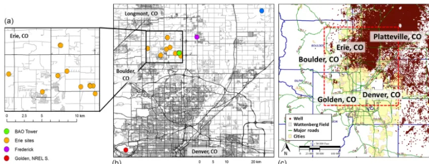
measurements taken at the Golden National Renewable En-ergy Laboratory (NREL), Frederick, and Platteville. All Col-orado sites are shown in Fig. 2.
Shown in Fig. 2 are the boundaries of the Wattenberg Gas Field and all active and inactive wells. In general, oil and gas activity increases in density moving from the southwest-ern side of the deployment region to the northeastsouthwest-ern side, with the Erie sites on the edge of the gas field. Note that the Golden site has no nearby oil and gas activity, while the Platteville site is surrounded by a high density of wells. The pods were sited in rural and suburban areas primarily at homes, schools, or in open spaces with two monitors sited at a water reclamation facility. Of the 18 monitors, data from 15 were included in the following analysis. Three monitors were excluded because of extended power failure, temperate or humidity sensor failure, or MOx VOC sensor malfunction. Some of the remaining 15 monitors experienced occasional power loss, but all necessary sensors operated continuously.
In Los Angeles, we partnered with two community-based organizations, Redeemer Community Partnership and Esper-anza Community Housing, and deployed Y-Pods through-out a neighborhood sthrough-outh of downtown Los Angeles. This deployment lasted approximately 8 weeks. The community was specifically interested in deploying a monitoring net-work around an active oil extraction site. In this case, sites were selected at varying distances away from the drilling op-eration as well as varying distances from freeways, another
potential source of pollutants (Fig. 3). Thirteen of the sites were within an approximately 5×5 km grid, and two addi-tional sites were located further to the northwest and north-east. These two additional sites were utilized because they al-lowed for continuous co-location with reference instruments for validation purposes. The deployment area in Los Ange-les was primarily urban and suburban with high-density res-idential areas, some commercial and industrial land use, and much higher-density traffic than the Colorado deployment area.
Figure 2.Maps of Colorado deployment area with every site displayed in panel(b)and the Erie sites displayed in panel(a). Panel(c)indicates active and inactive wells in the Wattenberg Gas Field along with major urban areas and counties; data are courtesy of the Colorado Oil and Gas Conservation Commissions (COGCC, 2017).
Figure 3.Map of Los Angeles deployment sites, showing(a)the deployment area and all sites where co-locations with reference monitors occurred and(b)the distribution of monitoring sites in relation to major roadways and the drill site of interest (note the monitor locations have been approximated to the center of their respective blocks to protect participant identities).
crude oil (US EIA 2016b), and Los Angeles County is home to more than 5000 active oil wells (Sadd and Shamasunder, 2015). In both cases we expect methane to be emitted or co-emitted with other VOCs; we attempt to better understand local sources, methane may serve as a valuable indicator of emissions from these types of sites. The ratio of methane rel-ative to other combustion products such as CO and CO2will likely be higher from sites related to oil and gas activity than from other local sources such as traffic (Nam et al., 2004; Popa et al., 2014; Peischl et al., 2013). While the two de-ployment locations offer contrasting sampling environments,
both locations offer complexity in terms of number and types of sources, geography, and typical atmospheric trends.
2.3 Sensor signal processing
of current increases when the target gas (e.g., methane) is present, thus reducing the amount of oxygen adsorbed to the sensor’s surface (Figaro USA, Inc.). In other words, the resis-tance across the sensor decreases with increasing methane. In both the Y-Pods and U-Pods, the sensor voltage is continu-ously recorded to the SD card. Using Eq. (1), provided by the sensor manufacturer, we calculate the sensor resistance (Rs) at various concentrations (Figaro, 2005). In this equationVc is the circuit voltage,RLis the load resistance, andVoutis the logged voltage.R0represents the resistance in clean air and the ratio ofRs/R0is typically used in the analysis of MOx sensor data (Eugster and Kling, 2012; Piedrahita et al., 2014). Gas sensor signals, temperature, humidity, and pressure are recorded to the SD card approximately every 6–25 s (depend-ing on a pod’s programm(depend-ing). This frequent data acquisition allows for the use of minute-median data in calibration and analysis. Unless otherwise stated, this is the time resolution used in our analysis and shown in this paper.
Rs=
Vc×RL
Vout −RL (1)
2.4 Sensor calibration, validation, and analysis
Field normalizations were used to generate calibration mod-els for the sensors. Field normalization provides one ap-proach to correcting for the cross sensitivities that low-cost sensors tend to exhibit with respect to temperature, hu-midity, and other trace gases (Spinelle et al., 2015, 2017; Sadighi et al., 2018; Masson 2015a, b; Wang et al., 2010). This method is implemented by co-locating low-cost sensor systems with high-quality reference instruments (typically regulatory-grade monitors) for a given period and then gen-erating a calibration model using an approach such as lin-ear regression. These calibration models predict the methane concentration (in ppm) based on the sensor signal (Rs/R0) and other predictors. An advantage of calibrating sensors in the field as opposed to in a laboratory setting is that the mod-els will be trained for the pollutant levmod-els of interest and across the same dynamic temperature and humidity values that a sensor will likely experience during field deployment. In a study involving personal air quality monitors, Piedrahita et al. (2014) successfully calibrated sensors and provided sensor-specific uncertainty estimates using this method.
In Colorado, we co-located U-Pods with a Los Gatos cav-ity ring-down spectrometer operated by the Penn State Na-tive Trailer team at the Platteville Atmospheric Observatory in Platteville, CO. In Los Angeles, we co-located Y-Pods with reference instruments at two different sites. The pre-deployment co-location was with a Baseline Mocon Series 900 Methane/Non-methane Hydrocarbon Analyzer located in a primarily residential suburban area of Los Angeles. The post-deployment calibration was with a Picarro cavity ring-down spectrometer located in a suburban/urban area with a mix of residential, retail, and industrial land use. Reference instruments at both Los Angeles sites were operated by the
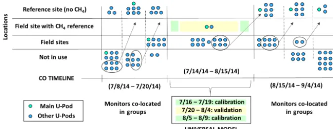
South Coast Air Quality Management District. The timelines in Figs. 4 and 5 illustrate when pods were co-located vs. de-ployed in the field and which data were used for the genera-tion of calibragenera-tion models (i.e., training data) versus the val-idation of those models (i.e., testing data). Note that for the Colorado deployment, both before and after the field deploy-ment, the monitors were co-located in batches due to logis-tical constraints. Arrows indicate the movement of batches of monitors, and the “not in use” row clarifies whether pods were deployed. In addition, during the Colorado deployment, a single calibration model (a universal model) was devel-oped based on the data from the “main” U-Pod, described in greater detail below. For the Los Angeles deployment, cali-bration models specific to each Y-Pod (sensor-specific mod-els) were used.
The setup of Y-Pods for these co-locations was governed by limitations at the site. In Colorado, Y-Pods were mounted to the railing of the Native Trailer (approximately 1.5 m above the trailer roof), which housed the reference instru-ments. The inlets to the reference instruments were approx-imately 2.5 m above the roof of the trailer and roughly 2 m away from the Y-Pods. For the first co-location in Los An-geles, the reference instrument was housed in a trailer in an open field. As we were not able to place the Y-Pods on the roof of the trailer, they were placed 0.75–1.5 m off the ground on the side of the trailer where the inlet was mounted. In this case, the Y-Pods were roughly 6 m below and 3 m to the side of the inlet. For the second co-location in Los Angeles, the reference instruments were housed inside of a building. In this case the Y-Pods were mounted to a railing roughly 1–2 m off the roof. However, the Y-Pods were also approximately 10 m away from and 1–2 m below the inlet, as this location was secure and out of the way of ongoing operations at the reference site. We would expect the variability between co-location setups to be most important for short-term spikes in CH4that do not pass over the Y-Pod and inlet evenly. As discussed in Sect. 3.1, our co-location site in Colorado expe-rienced the most short-term CH4spikes, whereas the changes in CH4concentration at the two LA sites were more gradual in nature.
Figure 4.Timeline for Colorado, indicating when monitors were co-located together in batches before and after the field deployment and il-lustrating how two U-Pods were sited with a reference instrument during the field deployment (these data were used for calibration generation or training data versus model validation or testing data).
Figure 5.Timeline for LA indicating when Y-Pods were co-located together with reference instruments before and after the field deployment, as well as which data were used for calibration generation (training data) versus model validation (testing data).
addition of environmental parameters, then interactions, and then transformations. Regression analysis provides sensor-specific coefficients for predictor variables. The models are then inverted so that gas concentration is expressed as a func-tion of sensor signals and can then be used to predict pol-lutant concentrations using new data collected in the field. This inverted model approach is typical for field normal-ization (Piedrahita et al., 2014; Spinelle et al., 2015, 2017). Evaluation of model performance was based on the coeffi-cient of determination (R2)and the root mean squared error (RMSE), as well as an analysis of the residuals in relation to relevant environmental and air quality parameters. Valida-tion data provide the opportunity to evaluate the consistency of each model’s performance based on the same metrics and the addition of mean bias.
Given the structure of each deployment and availability of co-located data, two different approaches to developing and applying calibration models were used: a universal calibra-tion model vs. sensor-specific models. For the Colorado de-ployment, a universal calibration model was developed us-ing the data from one sensor and this model were applied to all the sensors. As shown in Fig. 4, two U-Pods were co-located with the reference instrument throughout the field de-ployment. The data from one of these pods was used along with the following process: (1) generate a universal calibra-tion model using data from the main U-Pod co-located with the reference instrument; (2) normalize all of the other
U-Pods’ raw sensor signals to the main U-Pod using data from when they were co-located together before and after the field deployment; and (3) apply the universal calibration model to the normalized sensor data from each pod. The second U-Pod co-located with the reference instrument allows for val-idation of this method.
Table 2.Calibration models.
Model no. Description Model equation
1 Mdl1 Rs/R0=p1+p2(C)
2 Mdl3 Rs/R0=p1+p2(C)+p3(T )+p4(H )
3 Mdl4 Rs/R0=p1+p2(C)+p3(T )+p4(H )+p5(Ti)
4 Mdl4_1Int Rs/R0=p1+p2(C)+T (p3+p6(C))+p4(H )+p5(Ti)
5 Mdl4_2Int Rs/R0=p1+p2(C)+T (p3+p6(C))+p4(H )+p5(Ti)+p7(T×H ) 6 Mdl4_1Int_Tr Rs/R0=p1+p2(C)+T (p3+p6(C))+p4(ln(H ))+p5(Ti)
7 Mdl4_2Int_Tr Rs/R0=p1+p2(C)+T (p3+p6(C))+p4
H−1
+p5(Ti)+p7(T×H−1) 8 Mdl5_1Int Rs/R0=p1+p2(C)+T (p3+p6(C))+p4(H )+p5(Ti)+p7(Td)
9 Mdl5_2Int Rs/R0=p1+p2(C)+T (p3+p6(C))+p4(H )+p5(Ti)+p7(T×H )+p8(Td)
10 Mdl5_1Int_Tr Rs/R0=p1+p2(C)+T (p3+p6(C))+p4(ln(H ))+p5(Ti)+p7(Td)
11 Mdl5_2Int_Tr Rs/R0=p1+p2(C)+T (p3+p6(C))+p4
H−1+p5(Ti)+p7
T×H−1+p8(Td)
Predictors (lower casepwith subscripts):Cis pollutant concentration (ppm methane),Tis temperature,His absolute humidity,Tiis continuous time, andTdis
categorical time of day; Mdl indicates the number of predictors; Int indicates the number of interactions; Tr indicates use of transformations. The predictorp1
indicates an empirical constant.
3 Results and discussion
3.1 Differences in reference data and environmental conditions that impact calibration
Different sampling environments necessitate the use of dif-ferent strategies to produce the strongest calibration for each dataset. Reasons for this may be differences in local sources or metrological trends. Figure 6a and b illustrate the differ-ence in temperature and humidity values observed during calibration versus validation periods for both locations. In Colorado, the temperature and absolute humidity observed during the validation period are generally well represented by the data collected during the calibration period, although there are some high and low humidity values at certain tem-peratures that fall outside of the calibration parameter space. Conversely, in Los Angeles, the full range of temperature and humidity values observed during the validation period are captured in the calibration period. However, the Los Ange-les data have many temperature–humidity combinations that are unique to the validation period.
Other sensor limitations must be considered as well, for example relatively slow sensor response. A low-cost sen-sor with an operating principle relying on chemical reactions may not have time to fully detect a passing plume (Arfire et al., 2016), whereas this is not an issue for high-quality refer-ence instruments that rely instead on optical properties. The manufacturer of the Picarro cavity ring-down spectrometer, for example, cites a gas response time under 3 s (Picarro, Inc., 2015), while Baseline Mocon cites a response time of less than 5 s for the Series 900 Methane/Non-methane Hy-drocarbon Analyzer (Mocon, Inc., 2017). Given these quick response times and the high flow rates used for sampling by the reference instruments we would not expect a lag on the part of the reference instrument. The sensor failing to reach steady state when exposed to a short and high concentration
plume, as a result of slow sensor response, would be more of a concern for calibration. This limitation may result in sensor data that are fundamentally different from reference data, further complicating calibration model generation. One option for addressing this issue, explored below, is filtering short-duration reference data features prior to model genera-tion. Demonstrating the need for this step, Fig. 6d and e each show 3 days of data from the reference monitors in which the diurnal patterns are similar, but the Colorado data also in-clude short-term enhancements or “spikes” in methane pos-sibly from the oil and natural gas extraction activity in the study region. The histogram in Fig. 6c depicts the changes in methane values for each dataset from minute to minute, further highlighting instances in the Colorado data where methane levels change by 0.5 or even 1 ppm over the course of a minute. These differences in the environmental param-eter spaces emphasize the need to customize quantification methods to each dataset.
3.2 Comparing calibration models
Figure 6.Panels(a)and(b)are the temperature and humidity values observed during calibration and validation periods in Colorado and Los Angeles, respectively. Panel(c)is a histogram of the changes in methane from minute to minute (for the reference data) and panels(d)and (e)are 3 days of minute-resolution data from the reference instruments in Colorado and Los Angeles, respectively.
than twice the past hour’s standard deviation and last less than 5 min in duration.
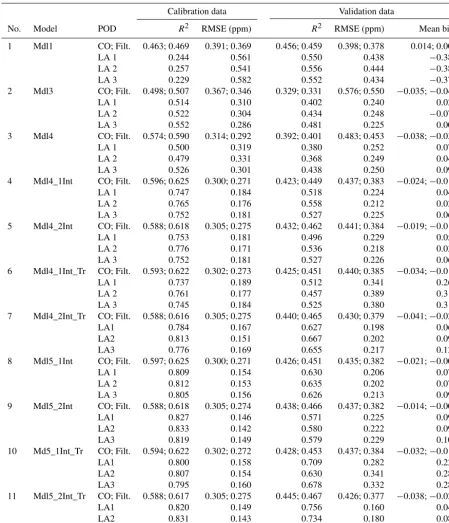
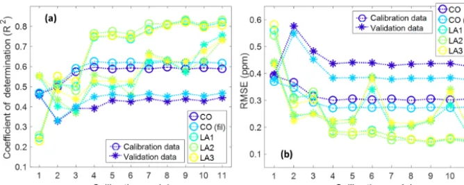
Figure 7a and b provide a graphical representation of the same statistics from Table 3 and emphasize the differences in results between the two datasets. For the Colorado data, the greatest improvement in fit was observed when time was added as a predictor, but then the results level off with no major improvements as the models increase in complexity. However, the results consistently returned a higher R2and lower RMSE when short-term methane spikes were filtered prior to model generation. In the Los Angeles dataset, there was continual improvement as models increased in complex-ity, with the most complex model producing a highR2and low RMSE as well as the most consistency across both the calibration and validations datasets.
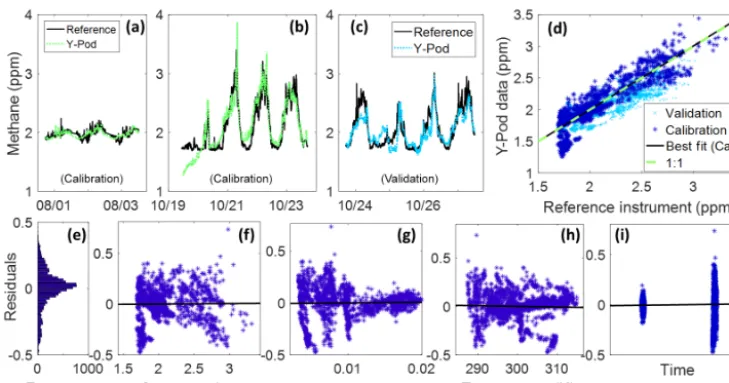
Figures 8 and 9 provide plots of the “best-fitting” calibra-tion models for each dataset based on regression statistics, consistency across calibration and validation data, and an analysis of the residuals. For the Colorado data, the selected model was the simplest well-fitting model, the fourth model, while for the Los Angeles data the selected model was the most complex model tested, the 11th model. With regards to both datasets, the selected model produced the most normal residuals, which also did not exhibit major trends in relation to the predictors, and they resulted in the closest one-to-one relationship between the fitted sensor data and the reference data. The time series plots also display the performance of the calibration model on the validation dataset.
As demonstrated by these two datasets, calibration mod-els are not “one size fits all”. While the deployments in Los Angles and Colorado occurred at roughly the same time of year, the best-fitting calibration models and regression re-sults proved to be quite different. This speaks to the need to consider the environmental and pollutant parameter space both when planning a deployment and when processing data. For example, more complex temperature and humidity be-havior may require more complex corrections. Additionally, if there is little overlap between conditions observed during calibration, validation, and field deployment then the result-ing calibrations will be less dependable. Likely, there are
factors beyond environmental parameter space driving dif-ferences between sensor and reference data. In that vein, it is important to explore the operational differences between the reference instrument and the sensors, including distance apart and proximity to significant sources. Here, we compen-sated for those operational differences by filtering “spikes” from the reference data; another modification could be to use a different averaging time such as hourly instead of minute data. This analysis demonstrates the importance of explor-ing different models, transformations of variables, and treat-ments of the data to find the model that provides the strongest methane estimates.
Table 3.Calibration model generation and validation results.
Calibration data Validation data
No. Model POD R2 RMSE (ppm) R2 RMSE (ppm) Mean bias
1 Mdl1 CO; Filt. 0.463; 0.469 0.391; 0.369 0.456; 0.459 0.398; 0.378 0.014; 0.007
LA 1 0.244 0.561 0.550 0.438 −0.381
LA 2 0.257 0.541 0.556 0.444 −0.388
LA 3 0.229 0.582 0.552 0.434 −0.379
2 Mdl3 CO; Filt. 0.498; 0.507 0.367; 0.346 0.329; 0.331 0.576; 0.550 −0.035;−0.040
LA 1 0.514 0.310 0.402 0.240 0.024
LA 2 0.522 0.304 0.434 0.248 −0.079
LA 3 0.552 0.286 0.481 0.225 0.003
3 Mdl4 CO; Filt. 0.574; 0.590 0.314; 0.292 0.392; 0.401 0.483; 0.453 −0.038;−0.035
LA 1 0.500 0.319 0.380 0.252 0.070
LA 2 0.479 0.331 0.368 0.249 0.045
LA 3 0.526 0.301 0.438 0.250 0.096
4 Mdl4_1Int CO; Filt. 0.596; 0.625 0.300; 0.271 0.423; 0.449 0.437; 0.383 −0.024;−0.011
LA 1 0.747 0.184 0.518 0.224 0.047
LA 2 0.765 0.176 0.558 0.212 0.026
LA 3 0.752 0.181 0.527 0.225 0.069
5 Mdl4_2Int CO; Filt. 0.588; 0.618 0.305; 0.275 0.432; 0.462 0.441; 0.384 −0.019;−0.011
LA 1 0.753 0.181 0.496 0.229 0.053
LA 2 0.776 0.171 0.536 0.218 0.035
LA 3 0.752 0.181 0.527 0.226 0.067
6 Mdl4_1Int_Tr CO; Filt. 0.593; 0.622 0.302; 0.273 0.425; 0.451 0.440; 0.385 −0.034;−0.019
LA 1 0.737 0.189 0.512 0.341 0.264
LA 2 0.761 0.177 0.457 0.389 0.316
LA 3 0.745 0.184 0.525 0.380 0.316
7 Mdl4_2Int_Tr CO; Filt. 0.588; 0.616 0.305; 0.275 0.440; 0.465 0.430; 0.379 −0.041;−0.027
LA1 0.784 0.167 0.627 0.198 0.061
LA2 0.813 0.151 0.667 0.202 0.096
LA3 0.776 0.169 0.655 0.217 0.120
8 Mdl5_1Int CO; Filt. 0.597; 0.625 0.300; 0.271 0.426; 0.451 0.435; 0.382 −0.021;−0.009
LA 1 0.809 0.154 0.630 0.206 0.076
LA 2 0.812 0.153 0.635 0.202 0.070
LA 3 0.805 0.156 0.626 0.213 0.095
9 Mdl5_2Int CO; Filt. 0.588; 0.618 0.305; 0.274 0.438; 0.466 0.437; 0.382 −0.014;−0.008
LA1 0.827 0.146 0.571 0.225 0.092
LA2 0.833 0.142 0.580 0.222 0.091
LA3 0.819 0.149 0.579 0.229 0.108
10 Md5_1Int_Tr CO; Filt. 0.594; 0.622 0.302; 0.272 0.428; 0.453 0.437; 0.384 −0.032;−0.018
LA1 0.800 0.158 0.709 0.282 0.225
LA2 0.807 0.154 0.630 0.341 0.285
LA3 0.795 0.160 0.678 0.332 0.281
11 Mdl5_2Int_Tr CO; Filt. 0.588; 0.617 0.305; 0.275 0.445; 0.467 0.426; 0.377 −0.038;−0.026
LA1 0.820 0.149 0.756 0.160 0.040
LA2 0.831 0.143 0.734 0.180 0.083
LA3 0.804 0.156 0.731 0.190 0.104
These models were then applied to normalized data from the other two Los Angeles Y-Pods included in the previous sec-tion. The raw sensor data from the Figaro TGS 2600 sensors were normalized using a simple linear regression (theR2 val-ues for these regressions were 0.989 and 0.999, respectively). Similar to the results from Sect. 3.2, the same model (MDL5_2INT_TR, model 11) emerges as the strongest for
Figure 7.PlottedR2(a)and RMSE(b)for all models; circle markers indicate results from calibration generation (using the training data) and asterisk markers indicate results from the application of the models to the validation data (or testing data).
Figure 8. “Best-fitting” model (MDL4_1INT) for the Colorado data with residual analysis (for validation data, RMSE is 0.383 ppm and mean absolute percent error is 12.13 %). Panels(a–c)are time series of the reference data and converted sensor data. Panel(d)is a scatter plot of the same data. Panels(e–i)are the residuals from the calibration generation.
to cover a larger environmental parameter space. This might also explain why the results for the “best-fitting” model are better for the validation period, which is much shorter. In any case, this calibration model approach provides useful infor-mation regarding methane levels (e.g., diurnal trends), as is demonstrated by Fig. 10, and this method can be used to con-vert the normalized signals from other sensors to a ppm value when logistics limit the potential for co-locating all sensors, whether due to time constraints or the limited availability of power and/or space at a co-location site. As the logistics of the Colorado deployment did not allow for sensor-specific calibrations, the universal calibration model approach is used below in Sect. 3.5 to convert the Colorado field data from all the U-Pods.
3.4 Further sensor quantification considerations Comprehensive best practices to guide the use of low-cost air quality sensors have not been established. A recent workshop
for low-cost sensors outlined some of the concerns shared throughout the research community including deployment logistics, data formatting and sharing, and communication of uncertainty (Clements et al., 2017). With our datasets, we investigated three issues related to the development of best practices: the length of a co-location for a field normaliza-tion, additional dataset-specific filtering based on environ-mental parameters, and cross sensitivities to non-methane pollutants.
3.4.1 Length of co-location
differ-Figure 9.“Best-fitting” model (Mdl5_2Int_Tr) for the Los Angeles data with residual analysis (LA1 shown) (for validation data, RMSE is 0.160 ppm and mean absolute percent error is 5.75 %). Panels(a–c)are time series of the reference data and converted sensor data. Panel (d)is a scatter plot of the same data. Panels(e–i)are the residuals from the calibration generation.
Table 4.Calibration and validation results for the universal calibration method (∗– normalized Y-Pod data).
Calibration data Validation data
R2 RMSE R2 RMSE Mean bias
MDL1 (1) LA1 0.154 0.493 0.209 0.856 −0.396
LA2∗ 0.223 0.835 −0.382
LA3∗ 0.201 0.836 −0.377
MDL3 (2) LA1 0.500 0.214 0.404 0.565 −0.249
LA2∗ 0.438 0.581 −0.292
LA3∗ 0.419 0.548 −0.256
MDL4 (3) LA1 0.496 0.215 0.397 0.577 −0.261
LA2∗ 0.434 0.589 −0.304
LA3∗ 0.412 0.560 −0.268
MDL4_1INT (4) LA1 0.463 0.230 0.372 0.622 −0.283
LA2∗ 0.411 0.624 −0.324
LA3∗ 0.387 0.606 −0.288
MDL5_2INT_TR (11) LA1 0.477 0.223 0.486 0.334 −0.098
LA2∗ 0.532 0.348 −0.139
LA3∗ 0.529 0.336 −0.129
ent models were tested with 20 iterations for each model. The resulting statistics are plotted in Fig. 11 along with error bars for±1 standard deviation.
The simplest model (Mdl1), using only sensor signal and no environmental predictors, seems to perform consistently well for all lengths of time; however, the residuals reveal strong trends with temperature and humidity, indicating that these variables are not being corrected for. Given the analy-sis of the residuals, this model may provide useful informa-tion, but its implementation is also likely to be misleading. For example, this model may be useful in applications that do not require detailed analysis or decision making based on the data, such as education and outreach in a K-12 classroom
pro-Figure 10.Time series of the universal calibration model (for MDL5_2INT_TR) generated using the Validation 2 period(b)and the ap-plication of the model to the pre- and post-deployment co-location data (aandc) for Y-Pods LA1 and the normalized data from LA2 and LA3.
Figure 11.R2(a)and RMSE(b)for the calibration model generation (based on a given length of time) and the application of those models to the complete Colorado data. Note that calibration data, or training data, are selected using a random stating point in the complete Colorado dataset and the appropriate amount of consecutive data. The colors indicate the model, and solid lines indicate calibration results while dashed lines indicating validation results.
vide a better calibration model, a sufficient amount of data must be used to avoid overfitting. Simply stated, the model selection should be appropriate to the data’s characteristics and intended purpose.
3.4.2 The impact of model extrapolation
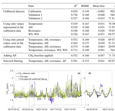
The additional co-located data from Los Angeles (Validation 2) facilitate a more in-depth exploration of the outlier resid-uals and approaches that could improve the predictive power of the calibration model. For example, dataset-specific filters were applied to remove values where extrapolation is likely occurring in field data. Extrapolation in this case would be in-stances where one or more predictors are outside of the range of values used to train the calibration model. Table 5 provides the statistics that result from applying the calibration model with and without this added filtering. The unfiltered dataset statistics are the same results explored in Sect. 3.2. All other
statistics in the table were calculated after values not ob-served during calibration were removed. In the first filtered grouping in Table 5, instances where individual temperature or humidity values (primarily extreme values) not observed were removed. In the second grouping, all data combinations not observed during calibration were removed, meaning all instances where exact combinations of temperature, humid-ity, etc. were not observed. The final filtering option, shown in the fourth section, applies knowledge of atmospheric com-position to assist with filtering. In this instance, the atmo-spheric baseline of methane was used to filter out low con-centration values; the baseline was determined by the mini-mum value observed in the CH4reference data.
processing being used to reduce negative values (Hagler et al., 2011) and examples of guidelines to remove negative values below a given threshold (US EPA, 2016). For work with sensor data, if the focus of the analysis is to under-stand enhancements over background captured by sensors, then removing improbably low values can elucidate these re-sults. If preliminary data are being shared with the public, then flagging and removing improbable values can reduce confusion. Given the challenges in sensor quantification, this second example in particular warrants consideration by those using sensors in partnership with communities. However, it is also likely that these underestimations contain valuable infor-mation about sensor behavior and sensitivity; removing these values will also introduce a negative bias to the data. Accord-ingly, when using this type of processing, researchers will need to be clear about why this approach is useful and valid. For this dataset, every instance where underestimations are removed by the filter coincides with days having a dynamic range of methane less than the expected uncertainty for the sensor, which indicates that these underestimations may be connected to a limit of detection issue. Figure B1 (Appendix B) demonstrates this association.
Additional filtering at nearly each stage yields some im-provement in statistics, with the removal of the complete data combinations not seen during calibration resulting in the largest improvements, but this method also removes a large portion of the data. The combination of applied knowledge of atmospheric composition and the removal of extreme indi-vidual values not observed during calibration yields improve-ments while maintaining a substantial amount of the data. This result, labeled “selected filtering”, suggests that this more conservative version of filtering may be sufficient. Not only did this filtering result in a RMSE that is lower than the RMSE for first validation dataset (0.1525 and 0.1601 ppm, respectively), but also these improvements are visible in a plot of the data. Figure 12a provides an overview of the complete dataset and highlights where some of the under-predictions are corrected for before 7 and 17 September, likely driven by the filter utilizing atmospheric principles. Figure 12b shows a close-up of a couple of days illustrating a reduction in overprediction, driven by the filter for either temperature, humidity, or resistance values.
As was demonstrated with the Validation 2 dataset, we ex-pect that applying the same filtering to each deployed sen-sor’s data should result in more reliable field data from all of the sites. Thus in addition to filtering data prior to cali-bration by removing short-duration enhancements in the ref-erence data, filtering converted sensor data can improve the reliability of calibrated data. While the bounds for this type of filtering should be dataset-specific, this step could easily be an automated addition to low-cost sensor quantification procedures.
3.4.3 Sensor cross sensitivities
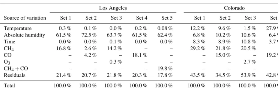
Another common concern for low-cost sensors is cross sen-sitivities to other gases, in addition to known cross sensitiv-ities to environmental factors. As discussed by Eugster and Kling (2012), the Figaro TGS 2600 sensor is reported to be sensitive to carbon monoxide as well as a few other hydrocar-bons (Figaro, 2005). This is not surprising, as each of these species can act as a reducing gas at the sensor surface and therefore also reduce the resistance to electron flow. While Eugster and Kling (2012) did not examine CO specifically given the absence of potential sources in their deployment area, they did perform an analysis of variance examining the effects of CO2and found no significant impacts. We applied the same analysis techniques to minute-resolution data to ex-amine the impacts of other gases, specifically CO, O3, and a few VOCs. Given the information provided by the sensor manufacturer, we expected a cross sensitivity to CO, but not to O3; this analysis provided an opportunity to check these assumptions. Table 6 includes the resulting explained vari-ance from each ANOVA, all of which included environmen-tal parameters and time along with the following differences: set 1 is CH4only, set 2 is CH4 and CO, set 3 is CH4 and O3, set 4 is CO only, and set 5 is the combined (CH4+CO) predictor.
represented in the AH 0.529 0.166 0.031 71 551
calibration data Resistance 0.548 0.160 0.028 70 851
WS, WD 0.526 0.167 0.031 69 578
Using only paired Temperature, AH, resistance 0.552 0.160 0.026 69 473
values seen in the Temperature, AH 0.564 0.157 0.030 51 233
calibration data Temperature, AH, resistance 0.574 0.160 0.063 20 059 Temperature, resistance, WS, WD 0.715 0.188 0.091 7645
Adding AP CH4baseline applied 0.552 0.160 0.047 71 736
Selected filtering Temperature, AH, resistance, AP 0.581 0.153 0.041 69 473
Figure 12. Panel(a)includes the complete Validation 2 dataset from the Los Angeles deployment. The statistics for each are RMSE is 0.17 ppm and absolute percent relative error is 6.77 % for the unfiltered data (blue); RMSE is 0.15 ppm and absolute percent relative error is 6.19 % for the filtered data (green), with the reference data plotted in black. Panel(b)is a close-up of approximately 2 days illustrating an instance where the filtering helped to reduce an overprediction of methane concentrations.
CO and CH4 allows us to examine the impacts of the CO cross sensitivity more closely. Figure 14 shows a portion of the Colorado data with both reference and U-Pod methane plotted along with carbon monoxide data from a reference monitor. In Fig. 14a spikes in CO correspond with overpre-dictions of methane (most notably on 8 August) and the scat-ter plot in Fig. 14b highlights how overpredictions seem to coincide with elevated CO concentrations.
In addition to this observed cross sensitivity to CO, we ex-pect that other hydrocarbons may affect the sensor response as well. This would be an important consideration for mea-surements made in areas with oil and gas activity where the pollutant mixtures may be complex. At the PAO site there was also a proton-transfer-reaction quadrupole mass spec-trometry (PTR-QMS) providing speciated VOC measure-ments (Halliday et al, 2016). Future work will provide a more
Table 6.Explained variance from ANOVA analyses on Figaro TGS 2600 resistance values (R/R0)for different parameter sets.
Los Angeles Colorado
Source of variation Set 1 Set 2 Set 3 Set 4 Set 5 Set 1 Set 2 Set 3 Set 4
Temperature 0.3 % 0.1 % 0.0 % 0.2 % 0.08 % 12.2 % 9.6 % 1.5 % 27.9 %
Absolute humidity 61.5 % 72.5 % 63.7 % 61.5 % 62.4 % 6.8 % 10.2 % 10.6 % 6.4 %
Time 0.0 % 0.0 % 0.1 % 0.0 % 0.0 % 8.3 % 8.9 % 10.8 % 3.7 %
CH4 16.8 % 2.6 % 14.2 % – – 29.2 % 21.8 % 20.5 % –
CO – 4.2 % – 18.1 % – – 15.0 % – 19.2 %
O3 – – 0.3 % – – – – 2.7 % –
CH4+CO – – – – 19.8 % – – – –
Residuals 21.4 % 20.7 % 21.8 % 20.3 % 17.8 % 43.5 % 34.5 % 53.9 % 42.8 %
Total 100.0 % 100.0 % 100.0 % 100.0 % 100.0 % 100.0 % 100.0 % 100.0 % 100.0 %
Figure 13.Histogram of carbon monoxide data from the two de-ployments and scatter plot of carbon monoxide data vs. methane data also from the two deployments. Note that all data in these two plots are from reference instruments.
explained by the residuals is at its lowest and the variance ex-plained by methane is at 10.1 %, higher than the percentages for the individual hydrocarbons. Thus, the Figaro TGS 2600 sensor seems to be cross sensitive to carbon monoxide and some hydrocarbons, effects that should be considered or mit-igated in future uses of this sensor to estimate methane.
Despite sampling in more complex environments than pre-vious deployments of this sensor (Eugster and Kling, 2012), we are still seeing a sizable proportion of the sensor data’s variance explained by ambient methane concentrations. Al-though these cross sensitivities need to be addressed to dis-cern which signals are driven by methane versus other pol-lutants, the Figaro TGS 2600 sensors are reacting in part to changes in ambient methane again providing useful methane estimates for applications where methane concentrations are needed with resolutions on the order of 0.2–0.4 ppm. Given the variety of low-cost sensors available, using the Figaro TGS 2600 sensors in a sensor array could provide addi-tional signals at each deployment site facilitating more
re-liable data. Including multiple sensor signals in a neural net-work calibration approach may also improve the accuracy of the calibrated data (Zimmerman et al., 2018; De Vito et al., 2008; Huyberechts et al., 1997). Future analysis of the data collected in Los Angeles and continued use of this sensor in areas with complex mixtures will require carbon monoxide and non-methane hydrocarbon impacts be considered.
3.5 Ability to assess spatial variability in the northern front range of Colorado
Figure 14. (a)Time series of methane and carbon monoxide data from the reference monitors and converted U-Pod sensor data.(b)Scatter plot of reference methane data (xaxis) vs. U-Pod methane data (yaxis) with the points colored by carbon monoxide vales. Together they further show the Figaro TGS 2600’s cross sensitivity to carbon monoxide, illustrating how many over predictions correspond to instances when CO is at or above 0.5 ppm.
Table 7.Explained variance of the Figaro TGS 2600 resistance values (R/R0)for parameter sets including different VOCs.
Source of variation Set 1 Set 2 Set 3 Set 4 Set 5 Set 6 Set 7
Temperature 9.6 % 17.4 % 10.1 % 10.9 % 33.7 % 28.9 % 16.3 %
Absolute humidity 10.2 % 11.7 % 14.2 % 7.5 % 6.2 % 9.0 % 12.6 %
Time 8.9 % 4.5 % 9.2 % 4.4 % 3.0 % 2.8 % 5.8 %
CH4 21.8 % 12.3 % 14.2 % 18.5 % – – 10.1 %
CO 15.0 % 13.6 % 14.4 % 19.7 % – 9.8 % 11.4 %
Acetaldehyde – 7.5 % – – 13.4 % 8.9 % 6.5 %
Benzene – – 4.6 % – 8.4 % 6.4 % 4.0 %
Methanol – – – 0.9 % 0.4 % 0.1 % 0.3 %
Residuals 34.5 % 33.0 % 33.4 % 38.2 % 34.9 % 34.1 % 33.2 %
Total 100.0 % 100.0 % 100.0 % 100.0 % 100.0 % 100.0 % 100.0 %
and were operated for the same amount of time throughout the deployment. The final step in preparing these data was to filter out data where the temperature and humidity val-ues were outside of those ranges observed during calibration and to remove data where concentration values were lower than an expected minimum (atmospheric background) was observed, similar to the analysis in Sect. 3.4.2. In this case a conservative 1.6 ppm was used, roughly half of our RMSE below background methane levels. For this analysis, filter-ing out implausibly low values highlights the differences in methane enhancements between the field sites. The largest amount of data removed from any U-Pod dataset as a result of this filtering was approximately 6 %.
Table 8 presents statistics illustrating the correlation efficients and RMSE for converted sensor data during co-location versus field deployment for both the 2 U-Pods con-tinuously paired and the mean of all 15 U-Pods. The result is high correlation when pods are co-located and low corre-lation when U-Pods are deployed to their field sites, high-lighting that (1) there is consistency in the data provided through the universal calibration model and (2) we are see-ing quite a bit of variability across the field sites.
Addition-ally, the RMSE for co-located U-Pods is less than the error we expect given the RMSE of 0.3832 ppm for the validation dataset. The details of each individual sensor versus P1 are available in Fig. A1 and Table A1, in Appendix A. These de-tails demonstrate the extent of inter-sensor variability for co-located sensors and the increase in variability for deployed sensors. While there is some variability among correlation coefficients, for nearly all sensors the periods of enhanced methane fall along the 1:1 line and most offsets occur at lower methane concentrations. Additionally, all RMSEs for co-located sensor fall below our expected uncertainty, while the RMSEs for deployed sensors is larger than this uncer-tainty (with the exception of the P1–P2 pair, which was co-located during the deployment).
Table 8.Statistics for Colorado data converted using the universal model method.
Post-co-location Deployed to field sites
R RMSE (ppm) R RMSE (ppm)
Co-located pair; P2 to P1 0.961 0.210 0.904 0.241
Mean of all U-Pods to P1 0.866 0.180 0.025 0.556
Figure 15.Time series of minute-resolution data from four Colorado sites and a map showing the location of the four U-Pod with respect to all active and inactive wells (COGCC, 2017).
Figure 16.Box plots of all data for each U-Pod, grouped into day-time and nightday-time values. Note that whiskers are the 5th and 95th percentile values. These U-Pods are then further grouped by region.
small time frame of data, we can see major differences be-tween the sites. For example, there was a clear diurnal trend with elevated methane each night at the Platteville site. The high time resolution also allows us to observe short-term day-time increases at different sites, which were more sporadic and likely due to local emissions as there is typically more atmospheric mixing in the daytime (Bamberger et al., 2014). In contrast, the Golden site (U-Pod G1) exhibited relatively little variability in methane with differences between this site and the others well above our RMSE, suggesting significant differences in methane concentrations between these sites. Figure 15b provides a reminder of where the oil and gas wells of the Wattenberg Field are in relation to these U-Pods. These
high-resolution data (minute-median) allow for the study of individual emission events and possibly their correlation to nearby activity or regional trends.
Figure 16 shows the day and night methane concentra-tions for each site throughout the deployment, grouped by re-gion. This figure also highlights the ambient background for methane±the U-Pod RMSE (0.3832 ppm) for this dataset on either side to illustrate that the enhancements above back-ground were well beyond our expected error. The sensor in Golden (U-Pod G1) exhibited little variability across both daytime and nighttime values, whereas all the sites in Erie, Frederick, and Platteville exhibited larger ranges and larger nighttime increases in methane likely contributed to by lo-cal or regional sources. At the majority of sites, over 50 % of the data fell within the RMSE of typical background levels of methane. Though the middle 50 % of the nighttime data appears slightly shifted upward for U-Pods E11 and E3 in Erie (the two pods located near the water reclamation facil-ity). This trend was even more pronounced at the sites in Frederick and Platteville. Recall the well density show in Figs. 2 and 15, illustrating no oil and gas activity around Golden, whereas we see higher-density activity in Erie and Frederick, with the highest density of activity around Plat-teville suggesting that one possible source driving this ele-vated methane is emissions from oil and gas activity. We ob-serve this trend at night when atmospheric mixing is more limited and the planetary boundary layer is lower.
Figure 17.Well sites (COGCC, 2015) are plotted along with the differences between the 90th percentile value for the main Platteville U-Pod (P1) and every other U-Pod during the day(a)and night(b). The color bar indicates the magnitude of the difference in units of ppm CH4, and the same color bar scale is applied to both plots.
Figure 18.Mean methane value for each hour of the day, for each U-Pod, grouped and color-coded by region.
(P1) and all other U-Pods during the day (left) versus at night (right). The daytime differences are small, within±0.2 ppm for all sites, possibly indicating effective daytime mixing. However, at night there is a clear gradient across the sites with little difference between the pods in Platteville and in-creasing differences as we move to the edge of the gas field and outside of it, with an approximately 1 ppm difference for the Golden site and the site furthest west in Erie. Throughout the Erie field sites, the two U-Pods furthest north show the smallest difference with the Platteville pods after the Freder-ick pod, which was located much further into the gas field. These two pods were also the ones located at the water recla-mation facility and therefore subject to an additional local methane source. Interestingly, however, the U-Pod furthest west in the Erie area was the only U-Pod in that grid lo-cated on the west side of the county line. This placed the pod in Boulder County during a time when a moratorium be-ginning in 2012 was in effect (Boulder County, 2017). This moratorium severely limited new oil and gas development in the county. Although we cannot conclusively say the ob-served difference in 90th percentile nighttime values is the result of differing methane trends on either side of the county
line, it is an indication of a question possibly worth revisiting using other data collected during the FRAPPE/DISCOVER-AQ campaigns. More importantly, this example demonstrates how low-cost sensors can offer preliminary or supplementary data to help inform and guide future work.
4 Conclusions
A common response to the question, “How good is low-cost sensor data?” is “it depends”. It depends on what question you are trying to answer, what data you intend to collect, how you would like to use the data, and what supporting measurements are available. As demonstrated by the quan-tification system applied to the two deployments examined in this paper, the use of low-cost sensors, certainly in the short-term, is likely to be heavily application-dependent and sen-sors should be calibrated and quantified to meet the needs of a given research question and in response to the conditions of a particular deployment. As low-cost sensor systems become easier to deploy and data processing becomes more auto-mated, these systems have tremendous potential. Their low-cost and portable nature allows for quick deployment across varied spatial scales, especially small, localized scales. Sen-sor data can already highlight potential “hotspots”, which could lead to better allocation of resources or the detection of potential air quality issues sooner. When used in this con-text, the sensor system described herein can provide a useful estimate of methane concentrations that may serve as pre-liminary or supplementary data. In Los Angeles, we were able to provide a methane prediction despite the complex-ity of sources and this methane signal has the potential to provide some insight into what is happening at the neighbor-hood level, although special attention will need to be paid to likely confounders and cross sensitivities. In Colorado, we were able to generate a dataset that can be examined on var-ious temporal and spatial scales as well as data able to char-acterize regional trends that concur with the observations of other researchers. While more research into cross sensitivi-ties and other deployment issues is certainly necessary, this sensor system currently provides a powerful tool for under-standing methane in communities near sources. Furthermore, this is a tool that is complementary to conventional monitor-ing methods.
Figure A1.Scatter plots of P1 versus every other Y-Pod including both co-located data (in green) and deployed data (in blue).
Table A1.Statistics for Colorado data converted using the universal model method, including data for each individual Y-Pod and statis-tics for each Y-Pod versus Y-Pod P1.
Co-located Deployed
R RMSE R RMSE
E1 0.914 0.117 −0.159 0.581
E2 0.940 0.084 −0.095 0.594
E3 0.909 0.284 0.168 0.619
E4 0.863 0.201 0.050 0.591
G1 0.737 0.200 −0.179 0.565
E5 0.849 0.132 0.054 0.529
P2 0.961 0.210 0.904 0.241
E6 0.847 0.166 −0.061 0.535
E7 0.864 0.124 −0.067 0.572
E8 0.931 0.336 −0.186 0.599
F1 0.819 0.182 0.221 0.550
E9 0.931 0.095 −0.454 0.655
E10 0.929 0.107 0.053 0.585
E11 0.624 0.208 0.104 0.571
Average 0.866 0.175 0.025 0.556
Appendix B: Sensor data underestimates and methane variability
Acknowledgements. Funding provided through the MetaSense Project (NSF Grant CNS-1446912), the AirWaterGas Project (NSF-SRN CBET: 1240584), and the DISCOVER-AQ Project (NASA). Thank you to all project partners during the DISCOVER-AQ/FRAPPE campaigns (NCAR, NOAA, CDPHE, US EPA), all project partners in Los Angeles at the University of Southern California Keck School of Medicine, Redeemer Community Part-nership (Nicole Wong), Sandy Navarro, William Flores, Esperanza Community Housing, and Occidental College. Additional thanks to all research and regulatory partners who assisted with site access and reference data: the NATIVE trailer team, Colorado Department of Public Health and the Environment, and South Coast Air Quality Management District. Thanks to Christine Wiedinmyer (CIRES) for the deployment maps included in this paper (Sect. 2.2). Thanks to all monitor site hosts in Colorado and Los Angeles, and current and former members of the Hannigan Research Lab, especially Nicholas Masson and Drew Meyers for their work on the U-Pod/Y-Pod hardware and software, and Evan Cof-fey and Kira Sadighi for their assistance with the deployment in LA.
Edited by: Dwayne Heard
Reviewed by: two anonymous referees
References
Allen, D. T.: Methane emissions from natural gas pro-duction and use: reconciling bottom-up and top-down measurements, Curr. Opin. Chem. Eng., 5, 78–83, https://doi.org/10.1016/j.coche.2014.05.004, 2014.
Adgate, J. L., Goldstein, B. D., and McKenzie, L. M.: Potential public health hazards, exposures and health effects from uncon-ventional natural gas development, Environ. Sci. Technol., 48, 8307–8320, https://doi.org/10.1021/es404621d, 2014.
Arfire, A., Marjovi, A., and Martinoli, A.: Mitigating slow dy-namics of low-cost chemical sensors for mobile air quality monitoring sensor networks. ESWN ’16 Proceedings of the 2016 International Conference on Embedded Wireless Systems and Networks, Conference Proceedings, 159–167, ISBN: 978-0-9949886-0-7, 2016.
Bamberger, I., Stieger, J., Buchmann, N., and Eugster, W.: Spatial variability of methane: attributing atmospheric concentrations to emissions, Environ. Pollut., 190, 65–74, https://doi.org/10.1016/j.envpol.2014.03.028, 2014.
Biaggi-Labiosa, A., Sola, F., Lebron-Colon, M., Evans, L. J., Xu, J. C., Hunter, G., Berger, G. M., and Gonzalez, J. M.: A novel methane sensor based on porous SnO2 nanorods: room
tem-in Navajo homes, Sci. Total Environ., 625, 608–618, https://doi.org/10.1016/j.scitotenv.2017.12.312, 2018.
Cheadle, L., Deanes, L., Sadighi, K., Casey, J. G., Collier-Oxandale, A., and Hannigan, M.: Quantifying neighborhood-scale spatial variations of ozone at open space and urban sites in Boul-der, Colorado using low-cost sensor technology, Sensors, 17, 9, https://doi.org/10.3390/s17092072, 2017.
Clements, A., Griswold, W., RS, A., Johnston, J. E., Hert-ing, M. M., Thorson, J., Collier-Oxandale, A., and Hanni-gan, M.: Low-cost air quality monitoring tools: from re-search to practice (a workshop summary), Sensors, 17, 2478, https://doi.org/10.3390/s17112478, 2017.
Collier, A., Knight, D., Hafich, K., Hannigan, M., Polmear, M., and Graves, B.: On the development and implementation of a project-based learning curriculum for air quality in K-12 schools, 2015 IEEE: Frontiers in Education Conference (FIE), Conference Pro-ceedings, https://doi.org/10.1109/FIE.2015.7344246, 2015. Colorado Oil and Gas Conservation Commission (COGCC), Wells,
data layer, available at: http://cogcc.state.co.us/documents/data/ downloads/gis/WELLS_SHP.ZIP (last access: 4 October 2017), 2015.
Colorado Oil and Gas Conservation Commission (COGCC): Online GIS Tool, available at: https://cogccmap.state.co.us/cogcc_gis_ online/, last access: 4 October 2017.
Cross, E. S., Williams, L. R., Lewis, D. K., Magoon, G. R., Onasch, T. B., Kaminsky, M. L., Worsnop, D. R., and Jayne, J. T.: Use of electrochemical sensors for measurement of air pollution: cor-recting interference response and validating measurements, At-mos. Meas. Tech., 10, 3575–3588, https://doi.org/10.5194/amt-10-3575-2017, 2017.
Davis K. J., Deng A., Lauvaux T., Miles N. L., Richardson S. J., Sarmiento D. P., Kevin R., Gurney, R., Hardesty, M., Bonin, T. A., Brewer, W. A., Lamb, B. K., Shepson, P. B., Harvey, R. M., Cambaliza, M. O., Sweeney, C., Turnbull, J. C., Whetstone, J., and Karion, A.: The Indianapolis flux ex-periment (INFLUX): a test-bed for developing urban green-house gas emission measurements, Elem. Sci. Anth. 5, 21, https://doi.org/10.1525/elementa.188, 2017.
De Vito, S., Massera, E., Piga, M., Martinotto, L., and Di Francia, G.: On field calibration of an electronic nose for benzene estima-tion in an urban polluestima-tion monitoring scenario, Sensor. Actuat. B-Chem., 129, 750–57, https://doi.org/10.1016/j.snb.2007.09.060, 2008.
DISCOVER-AQ: Database, https://doi.org/10.5067/Aircraft/DISCOVER-AQ/Aerosol-TraceGas, 2015.
Eugster, W. and Kling, G. W.: Performance of a low-cost methane sensor for ambient concentration measurements in preliminary studies, Atmos. Meas. Tech., 5, 1925–1934, https://doi.org/10.5194/amt-5-1925-2012, 2012.
Fang, Y., Naik, V., Horowitz, L. W., and Mauzerall, D. L.: Air pol-lution and associated human mortality: the role of air pollutant emissions, climate change and methane concentration increases from the preindustrial period to present, Atmos. Chem. Phys., 13, 1377–1394, https://doi.org/10.5194/acp-13-1377-2013, 2013. Figaro: TGS 2600 – for the detection of air contaminants, On-line
product data sheet, available at: http://www.figarosensor.com/ products/2600pdf.pdf (last access: 4 October 2017), 2005. Fiore, A. M., West, J. J., Horowitz, L. W., Naik, V., and
Schwarzkopf, M. D.: Characterizing the tropospheric ozone response to methane emission controls and the benefits to climate and air quality, J. Geophys. Res., 113, 2156–2202, https://doi.org/10.1029/2007JD009162, 2008.
Hagler, G. S. W., Yelverton T. L. B., Vedantham, R., Hansen, A. D. A., and Turner, J. R.: Post-processing method to reduce noise while preserving high time resolution in aethalometer real-time black carbon data, Aerosol Air Qual. Res., 11, 539–546, https://doi.org/10.4209/aaqr.2011.05.0055, 2011.
Halliday, H. S., Thompson, A. M., Wisthaler, A., Blake, D., Horn-brook, R. S., Mikoviny, T., Muller, M., Eicher, P., Apel, E. C., and Hills, A. J.: Atmospheric benzene observations from oil and gas production in the Denver Julesburg basin in July and August 2014, J. Geophys. Res.-Atmos., 121, 11055–11074, https://doi.org/10.1002/2016JD025327, 2016.
Heimann, I., Bright, V. B., McLeod, M. W., Mead, M. I., Popoola, O. A. M., Stewart, G. B., and Jones, R. L.: Source attribution of air pollution by spatial scale separation using high spatial density networks of low cost air quality sensors, Atmos. Environ., 113, 10–19, https://doi.org/10.1016/j.atmosenv.2015.04.057, 2015. Helmig, D., Thompson, C. R., Evans, J., Boylan, P., Hueber, J., and
Park, J. H.: Highly elevated atmospheric levels of volatile organic compounds in the uintah basin, Utah, Environ. Sci. Technol., 48, 4707–4715, https://doi.org/10.1021/es405046r, 2014.
Huyberechts, G., Szeco, P., Roggen, J., and Licznerski, B. W.: Simultaneous quantification of carbon monoxide and methane in humid air using a sensor array and an artifi-cial neural network, Sensor. Actuat. B-Chem., 45, 123–30 https://doi.org/10.1016/S0925-4005(97)00283-9, 1997. Intergovernmental Panel on Climate Change (IPCC): Climate
Change 2014 Synthesis Report, available at: https://www.ipcc. ch/pdf/assessment-report/ar5/syr/SYR_AR5_FINAL_full.pdf (last access: 4 October 2017), ISBN: 978-92-9169-143-2, 2015. Karion, A., Sweeney, C., Pétron, G., Frost, G., Hardesty, R. M.,
Kofler, J., Miller, B. R., Newberger, T., Wolter, S., Banta, R., Brewer, A., Dlugokencky, E., Lang, P., Montzka, S. A., Schnell, R. S., Tans, P., Trainer, M., Zamora, R., and Conley, S.: Methane emissions estimate from airborne measurements over a western United States natural gas field, Geophys. Res. Lett., 40, 4393– 4397, https://doi.org/10.1002/grl.50811, 2013.
Kim, J., Shusterman, A. A., Lieschke, K. J., Newman, C., and Cohen, R. C.: The BErkeley Atmospheric CO2 Ob-servation Network: field calibration and evaluation of low-cost air quality sensors, Atmos. Meas. Tech., 11, 1937–1946, https://doi.org/10.5194/amt-11-1937-2018, 2018.
Kort, E. A., Frankenberg, C., Costigan, K. R., Lindenmaier, R., Dubey, M. K., and Wunch, D.: Four corners: the largest US methane anomaly viewed from space, Geophys. Res. Lett., 41, 6898–6903, https://doi.org/10.1002/2014GL061503, 2014. Lewis, A. C., Lee, J., Edwards, P. M., Shaw, M. D., Evans, M. J.,
Moller, S. J., Smith, K. R., Buckley, J. W., Ellis, M., Gillot, S. R., and White, A.: Evaluating the performance of low cost chemical sensors for air pollution research, Faraday Discuss., 189, 85–103, https://doi.org/10.1039/C5FD00201J, 2016.
Masson, N., Piedrahita, R., and Hannigan, M.: Approach for quan-tification of metal oxide type semiconductor gas sensors used for ambient air quality monitoring, Sensor. Actuat. B-Chem., 208, 339–345, https://doi.org/10.1016/j.snb.2014.11.032, 2015a. Masson, N., Piedrahita, R., and Hannigan, M.:
Quantifica-tion method for electrolytic sensors in long-term moni-toring of ambient air quality, Sensors, 15, 27283–27302, https://doi.org/10.3390/s151027283, 2015b.
Mead, M. I., Popoola, O. A. M., Stewart, G. B., Landshoff, P., Calleja, M., Hayes, M., Baldovi, J. J., McLeod, M. W., Hodgson, T. F., Dicks, J., Lewis, A., Cohen, J., Baron, R., Saffell, J. R., and Jones, R. L.: The use of electro-chemical sensors for monitoring urban air quality in low-cost, high-density networks, Atmos. Environ., 70, 186–203, https://doi.org/10.1016/j.atmosenv.2012.11.060, 2013.
Miller, S. M., Wofsy, S. C., Michalak, A. M., Kort, E. A., Andrews, A. E., Biraud, S. C., Dlugokencky, E. J., Eluszkiewicz, J., Fischer, M. L., Janssens-Maenhout, G., Miller, B. R., Miller, J. B., Montzka, S. A., Nehrkorn, T., and Sweeney, C.: Anthropogenic emissions of methane in the United States, P. Natl. Acad. Sci. USA, 110, 20018–20022, https://doi.org/10.1073/pnas.1314392110, 2013.
Mobile Sensing Technology: U-Pod open-source construction and parts information, available at: http://mobilesensingtechnology. com/, last access: 4 October 2017.
Mocon, Inc – Baseline: Series 9000 Total Hydrocarbon Ana-lyzer, available at: www.baseline-mocon.com (last access: 7 May 2018), 2017.
Moltchanov, S., Levy, I., Etzion, Y., Lerner, U., Broday, D. M., and Fishbain, B.: On the feasibility of measuring urban air pollution by wireless distributed sensor networks, Sci. Total Environ., 502, 537–547, https://doi.org/10.1016/j.scitotenv.2014.09.059, 2015. Moore, C. W., Zielinska, B., Petron, G., and Jackson, R. B.: Air
impacts of increased natural gas acquisition, processing, and use: a critical review, Environ. Sci. Technol., 48, 8349–8359, https://doi.org/10.1021/es4053472, 2014.
Nam, E. K., Jensen, T. E., and Wallington, T. J.: Methane Emis-sions from Vehicles, Environ. Sci. Technol., 38, 2005–2010, https://doi.org/10.1021/es034837g, 2004.
National Oceanic and Atmospheric Association (NOAA): Global Greenhouse Gas Reference Network: Trends in Atmospheric Methane, available at: https://www.esrl.noaa.gov/gmd/ccgg/ trends_ch4/#global_data, last access: 4 October 2017.